Appendix D
Discrete-time Dynamic Systems
This brief review is meant as a refresher for readers who are familiar with the topic. It summarizes those concepts that are used within the textbook. It also introduces the notations adopted in this book.
D.1 DISCRETE-TIME DYNAMIC SYSTEMS
A dynamic system is a system whose variables proceed in time. A concise representation of such a system is the state space model. The model consists of a state vector x(i) where i is an integer variable representing the discrete time. The dimension of x(i), called the order of the system, is M. We assume that the state vector is real-valued. The finite-state case is introduced in Chapter 4.
The process can be influenced by a control vector (input vector) u(i) with dimension L. The output of the system is given by the measurement vector (observation vector) z(i) with dimension N. The output is modelled as a memoryless vector that depends on the current values of the state vector and the control vector.
By definition, the state vector holds the minimum number of variables which completely summarize the past of the system. Therefore, the state vector at time i + 1 is derived from the state vector and the control vector, both valid at time i:
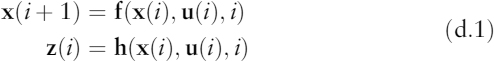
f(.) is a possible nonlinear vector function, the system function, that may depend explicitly on time. h(.) is the measurement function.
Note that if the time series ...
Get Classification, Parameter Estimation and State Estimation: An Engineering Approach Using MATLAB now with the O’Reilly learning platform.
O’Reilly members experience books, live events, courses curated by job role, and more from O’Reilly and nearly 200 top publishers.

