10.4 The Spherical Simplex Kalman Filter
Returning to (5.51), we can now write
(10.39) 
where from (10.38) we can identify the sigma points as
(10.40) ![]()
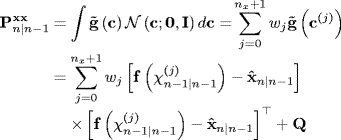
with ![]() defined by (10.34)–(10.36). In a manner similar to that of the UKF, we obtain the remaining predictive equations, with the state covariance given by
defined by (10.34)–(10.36). In a manner similar to that of the UKF, we obtain the remaining predictive equations, with the state covariance given by
(10.41) 
and the observation prediction equations
(10.42) ![]()
(10.43) ![]()
(10.44) ![]()
(10.45) 
where
(10.46) ![]()
Get Bayesian Estimation and Tracking: A Practical Guide now with the O’Reilly learning platform.
O’Reilly members experience books, live events, courses curated by job role, and more from O’Reilly and nearly 200 top publishers.

