Bayesian Estimation and Tracking: A Practical Guide

8.2 Multidimensional Finite Difference Kalman Filters

8.2.1 Multidimensional Finite Difference State Prediction

In manner similar to the approach taken in the one-dimensional case, we first repeat the multidimensional state prediction equation developed for the EKF given by (7.33)

(8.26)

Now, using the second-order finite difference term of multidimensional Stirling's polynomial given by equation (2.74) and letting x → c and x₀ = 0, (8.26) becomes

(8.27)

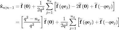
where e_j is a unit vector along the Cartesian axis of the j th dimension and q is a step size that must be finite, real, and greater than zero.

Defining

(8.28)

leads to the identities

(8.29)

and

(8.30)

Here, is a free parameter that determines the value of q. To maintain q as finite, real, and greater than zero, we must restrict to the ...