10 A REGRESSION MODEL FOR PERIODIC DATA
10.1 THE MODEL
A general periodic model is of the form, y(j) = μ + M · cos(2π[j/k + φ]), where j is integers indexing time. The mean, μ, shifts the function up and down, M changes the amplitude, and φ shifts (sometimes called the phase) the location of the maximum and minimum. The function repeats itself every k periods. For annual data, k would be 12 for monthly data and 52 for weekly data. Figure 10.1 displays the function y1(j) = 2 + 8 · cos(2π[j/12 + .25]) in solid lines and y2(j) = 4 + 4 · cos(2π[j/24 + .70]) in dashed lines.
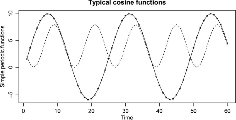
FIGURE 10.1 Cosine functions can vary in amplitude, mean, period, and phase.
The most basic periodic models are of the form y(j) = μ + M · cos(2π[j/k + φ]) + ϵj, where the errors are white noise. However, the time series may be more complex requiring a linear combination of periodic functions and the error may not be white noise.
For this most basic model, it is assumed that k is known, and μ, M, and φ must be estimated. The problem min ∑[y(j) − μ − M · cos(2π[j/k + φ])]2, where μ, M, and φ are unknown, is not an OLS (ordinary least squares) problem. Why (hint: take the partial derivatives and set them equal to zero)?
However, there is a trick that allows this to be solved as an OLS problem (Bloomfield, 2000). Let y(j) = μ + B · cos(2πj/k) + C · sin(2πj/k) where B = M · cos(2πφ) and C = −M · sin(2πφ). The ...
Get Basic Data Analysis for Time Series with R now with the O’Reilly learning platform.
O’Reilly members experience books, live events, courses curated by job role, and more from O’Reilly and nearly 200 top publishers.

