5.4 The Largest Component
In this section we assume α = 2, i.e., we work in binary n-cubes. All results and proofs easily extend to arbitrary alphabets. The analysis of large components presented here follows [20]. Section 5.3 has shown that the connectivity threshold ![]() reflects the disappearance of isolated vertices. Therefore, it seems natural to ask which probabilities we find a unique large component for. In addition, one would like to know its size. Note that the connectivity property alone is not sufficient for understanding the neutral evolution. The relevant property will be identified in Section 5.5 and is related to the emergence of short paths in n-cubes. Intuitively the largest component is in its “early” stage locally “treelike” and therefore not suited for preserving sequence-specific information. We set
reflects the disappearance of isolated vertices. Therefore, it seems natural to ask which probabilities we find a unique large component for. In addition, one would like to know its size. Note that the connectivity property alone is not sufficient for understanding the neutral evolution. The relevant property will be identified in Section 5.5 and is related to the emergence of short paths in n-cubes. Intuitively the largest component is in its “early” stage locally “treelike” and therefore not suited for preserving sequence-specific information. We set
![]()
and
![]()
We write a Qn2-vertex v=(x1,...,xn) as
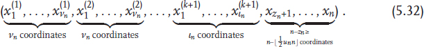
For any 1 ≤ s ≤ vn, r = 1,..., k we set e(r)s to be the s+(r–1)vn th-unit vector, i.e., e(r) has exactly one 1 at its (s+(r–1)vn)th coordinate. Similarly, let e(k+1)(s, 1 ≤ s ≤ ln, denote the(s + kvn)th-unit vector. We use the ...
Get Analysis of Complex Networks now with the O’Reilly learning platform.
O’Reilly members experience books, live events, courses curated by job role, and more from O’Reilly and nearly 200 top publishers.

