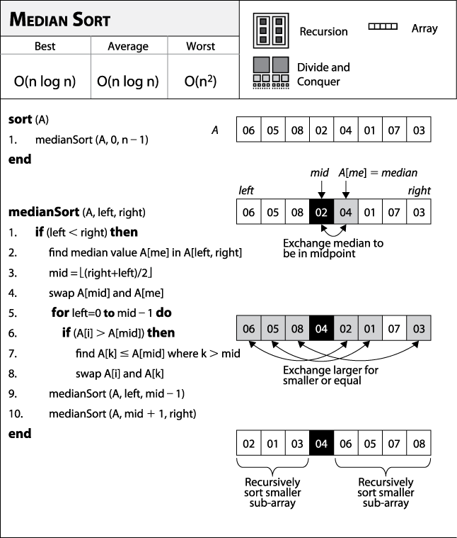
Divide and conquer, a common approach in computer science, solves a problem by dividing it into two independent subproblems, each about half the size of the original problem. Consider the Median Sort algorithm ( Figure 4-8) that sorts an array A of n≥1 elements by swapping the median element A[me] with the middle element of A (lines 2–4), creating a left and right half of the array. Median Sort then swaps elements in the left half that are larger than A[mid] with elements in the right half that are smaller or equal to A[mid] (lines 5–8). This subdivides the original array into two distinct subarrays of about half the size that each need to be sorted. Then Median Sort is recursively applied on each subarray (lines 9–10).
A full example of Median Sort in action is shown in Figure 4-9, in which each row corresponds to a recursive invocation of the algorithm. At each step, there are twice as many problems to solve, but each problem size has been cut in about half. Since the subproblems are independent of each other, the final sorted result is produced once the recursion ends.
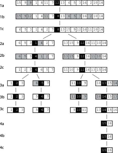
The initial unsorted array is shown in the line labeled 1a, and the selected median element, A[me], is identified by a gray square. A[me] is swapped (line 1b) with the midpoint element (shown in the black square), and the larger elements (shown as the gray squares in line 1b to the left of the midpoint) are swapped with the smaller or equal elements (shown as gray squares in line 1b to the right of the midpoint) to produce the divided array in line 1c. In the recursive step, each of the smaller subarrays is sorted, and the progress (on each subarray) is shown in lines 2a-2c, 3a-3c, and 4a-4c.
Context
Implementing Median Sort depends on efficiently selecting the median element from an unsorted array. As is typical in computer science, instead of answering this question, we answer a different question, which ultimately provides us with a solution to our original question. Imagine someone provided you with a function p = partition (left, right, pivotIndex), which selects the element A[pivotIndex] to be a special pivot value that partitions A[left, right] into a first half whose elements are smaller or equal to pivot and a second half whose elements are larger or equal to pivot. Note that left≤pivotIndex≤right, and the value p returned is the location within the subarray A[left, right] where pivot is ultimately stored. A C implementation of partition is shown in Example 4-3.
Example 4-3. C implementation to partition ar[left,right] around a given pivot element
/**
 * In linear time, group the subarray ar[left, right] around a pivot
 * element pivot=ar[pivotIndex] by storing pivot into its proper
 * location, store, within the subarray (whose location is returned
 * by this function) and ensuring that all ar[left,store) <= pivot and
 * all ar[store+1,right] > pivot.
 */
int partition (void **ar, int(*cmp)(const void *,const void *),
               int left, int right, int pivotIndex) {
  int idx, store;
  void *pivot = ar[pivotIndex];

  /* move pivot to the end of the array */
  void *tmp = ar[right];
  ar[right] = ar[pivotIndex];
  ar[pivotIndex] = tmp;

  /* all values <= pivot are moved to front of array and pivot inserted
   * just after them. */
  store = left;
  for (idx = left; idx < right; idx++) {
    if (cmp(ar[idx], pivot) <= 0) {
      tmp = ar[idx];
      ar[idx] = ar[store];
      ar[store] = tmp;
      store++;
    }
  }

  tmp = ar[right];
  ar[right] = ar[store];
  ar[store] = tmp;
  return store;
}
How can we use partition to select the median efficiently? First, let's review the results of this method, as shown on a sample unsorted array of 16 elements. The first step is to swap the pivot with the rightmost element. As the loop in partition executes, the key variables from the implementation are shown in Figure 4-10. store is the location identified by the circle. Each successive row in Figure 4-10 shows when the loop in partition identifies, from left to right, an element A[idx] that is smaller than or equal to the pivot (which in this case is the element "06"). Once there are no more elements smaller than or equal to pivot, the element in the last computed store is swapped with the rightmost element, thus safely placing the pivot in place.
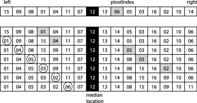
After partition(0,15,9) executes and returns the location p=5 of the pivot value, you can see that A[left, p) are all less than or equal to pivot, whereas A[p+1,right] are all greater than or equal to pivot. How has this made any progress in selecting the median value? Note that p is to the left of the calculated location where the median will ultimately end up in the sorted list (identified as the blackened array element labeled "median location"). Therefore, none of the elements to the left of p can be the median value! We only need to recursively invoke partition (this time with a different A[pivotIndex] on the right half, A[p+1,right]) until it returns p=median location.
Note that partition effectively organizes the array into two distinct subarrays without actually sorting the individual elements. partition returns the index p of the pivot, and this can be used to identify the kth element recursively in A[left, right] for any 1≤k≤right-left+1, as follows:
- if k=p+1
The selected pivot element is the kth value (recall that array indices start counting at 0, but k starts counting at 1).
- if k<p+1
The kth element of A is the kth element of A[left, p].
- if k>p+1
The kth element of A is the (k-p)th element of A[p+1,right].
In Figure 4-10, the goal is to locate the median value of A, or in other words, the k=8th largest element. Since the invocation of partition returns p=5, we next recursively search for the second smallest element in A[p+1,right].
Such a definition lends itself to a recursive solution, but it can also be defined iteratively where a tail-recursive function instead can be implemented within a loop (see the code repository for the example). selectKth is an average-case linear time function that returns the location of the kth element in array ar given a suitable pivotIndex; its implementation is shown in Example 4-4.
Example 4-4. selectKth recursive implementation in C
/**
 * Average-case linear time recursive algorithm to find position of kth
 * element in ar, which is modified as this computation proceeds.
 * Note 1 <= k <= right-left+1. The comparison function, cmp, is
 * needed to properly compare elements. Worst-case is quadratic, O(n^2).
 */
int selectKth (void **ar, int(*cmp)(const void *,const void *),
               int k, int left, int right) {
  int idx = selectPivotIndex (ar, left, right);
  int pivotIndex = partition (ar, cmp, left, right, idx);
  if (left+k-1 == pivotIndex) { return pivotIndex; }

  /* continue the loop, narrowing the range as appropriate. If we are within
   * the left-hand side of the pivot then k can stay the same. */
  if (left+k-1 < pivotIndex) {
    return selectKth (ar, cmp, k, left, pivotIndex-1);
  } else {
    return selectKth (ar, cmp, k - (pivotIndex-left+1), pivotIndex+1, right);
  }
}
The selectKth function must select a pivotIndex for A[left, right] to use during the recursion. Many strategies exist, including:
Select the first location (left) or the last location (right).
Select a random location (left≤random≤right).
If the pivotIndex repeatedly is chosen poorly, then selectKth degrades in the worst case to O(n2); however, its best- and average-case performance is linear, or O(n).
Forces
Because of the specific tail-recursive structure of selectKth, a nonrecursive implementation is straightforward.
Solution
Now connecting this discussion back to Median Sort, you might be surprised to note that selectKth works regardless of the pivotIndex value selected! In addition, when selectKth returns, there is no need to perform lines 5-8 (in Figure 4-8) of the Median Sort algorithm, because partition has already done this work. That is, the elements in the left half are all smaller or equal to the median, whereas the elements in the right half are all greater or equal to the median.
The Median Sort function is shown in Example 4-5 and is invoked on A[0,n−1].
Example 4-5. Median Sort implementation in C
/**
 * Sort array ar[left,right] using medianSort method.
 * The comparison function, cmp, is needed to properly compare elements.
*/
void mediansort (void **ar, int(*cmp)(const void *,const void *),
                 int left, int right) {
  /* if the subarray to be sorted has 1 (or fewer!) elements, done. */
  if (right <= left) { return; }

  /* get midpoint and median element position (1<=k<=right-left-1). */
  int mid = (right - left + 1)/2;
  int me = selectKth (ar, cmp, mid+1, left, right);

  mediansort (ar, cmp, left, left+mid-1);
  mediansort (ar, cmp, left+mid+1, right);
}
Consequences
Median Sort does more work than it should. Although the generated subproblems are optimal (since they are both about half the size of the original problem), the extra cost in producing these subproblems adds up. As we will see in the upcoming section on "Quicksort," it is sufficient to select pivotIndex randomly, which should avoid degenerate cases (which might happen if the original array is already mostly sorted).
Analysis
Median Sort guarantees that the recursive subproblems being solved are nearly identical in size. This means the average-case performance of Median Sort is O(n log n). However, in the worst case, the partition function executes in O(n2), which would force Median Sort to degrade to O(n2). Thus, even though the subproblems being recursively sorted are ideal, the overall performance suffers when considering n items already in sorted order. We ran Median Sort using a randomized selectPivotIndex function against this worst-case example where selectPivotIndex always returned the leftmost index. Ten trials were run, and the best and worst results were discarded; the averages of the remaining eight runs for these two variations are shown in the first two columns of Table 4-2. Observe that in the worst case, as the problem size doubles, the time to complete Median Sort multiplies more than fourfold, the classic indicator for O(n2) quadratic performance.
Table 4-2. Performance (in seconds) of Median Sort in the worst case
|
n |
Randomized pivot selection |
Leftmost pivot selection |
Blum-Floyd-Pratt-Rivest-Tarjan pivot selection |
|---|---|---|---|
|
256 |
0.000088 |
0.000444 |
0.00017 |
|
512 |
0.000213 |
0.0024 |
0.000436 |
|
1,024 |
0.000543 |
0.0105 |
0.0011 |
|
2,048 |
0.0012 |
0.0414 |
0.0029 |
|
4,096 |
0.0032 |
0.19 |
0.0072 |
|
8,192 |
0.0065 |
0.716 |
0.0156 |
|
16,384 |
0.0069 |
1.882 |
0.0354 |
|
32,768 |
0.0187 |
9.0479 |
0.0388 |
|
65,536 |
0.0743 |
47.3768 |
0.1065 |
|
131,072 |
0.0981 |
236.629 |
0.361 |
It seems, therefore, that any sorting algorithm that depends upon partition must suffer from having a worst-case performance degrade to O(n2). Indeed, for this reason we assign this worst case when presenting the Median Sort fact sheet in Figure 4-8.
Fortunately there is a linear time selection for selectKth that will ensure that the worst-case performance remains O(n log n). The selection algorithm is known as the Blum-Floyd-Pratt-Rivest-Tarjan (BFPRT) algorithm (Blum et al., 1973); its performance is shown in the final column in Table 4-2. On uniformly randomized data, 10 trials of increasing problem size were executed, and the best and worst performing results were discarded. Table 4-3 shows the performance of Median Sort using the different approaches for partitioning the subarrays. The computed trend line for the randomized pivot selection in the average case (shown in Table 4-3) is:
| 1.82*10−7*n*log (n) |
whereas BFPRT shows a trend line of:
| 2.35*10−6*n*log (n) |
Table 4-3. Performance (in seconds) of Median Sort in average case
|
n |
Randomized pivot selection |
Leftmost pivot selection |
Blum-Floyd-Pratt-Rivest-Tarjan pivot selection |
|---|---|---|---|
|
256 |
0.00009 |
0.000116 |
0.000245 |
|
512 |
0.000197 |
0.000299 |
0.000557 |
|
1,024 |
0.000445 |
0.0012 |
0.0019 |
|
2,048 |
0.0013 |
0.0035 |
0.0041 |
|
4,096 |
0.0031 |
0.0103 |
0.0128 |
|
8,192 |
0.0082 |
0.0294 |
0.0256 |
|
16,384 |
0.018 |
0.0744 |
0.0547 |
|
32,768 |
0.0439 |
0.2213 |
0.4084 |
|
65,536 |
0.071 |
0.459 |
0.5186 |
|
131,072 |
0.149 |
1.8131 |
3.9691 |
Because the constants for the more complicated BFPRT algorithm are higher, it runs about 10 times as slowly, and yet both execution times are O(n log n) in the average case.
The BFPRT selection algorithm is able to provide guaranteed performance by its ability to locate a value in an unordered set that is a reasonable approximation to the actual median of that set. In brief, BFPRT groups the elements of the array of n elements into n/4 groups of elements of four elements (and ignores up to three elements that don't fit into a group of size 4[9]). BFPRT then locates the median of each of these four-element groups. What does this step cost? From the binary decision tree discussed earlier in Figure 4-5, you may recall that only five comparisons are needed to order four elements, thus this step costs a maximum of (n/4)*5=1.25*n, which is still O(n). Given these groupings of four elements, the median value of each group is its third element. If we treat the median values of all of these n/4 groups as a set M, then the computed median value (me) of M is a good approximation of the median value of the original set A. The trick to BFPRT is to recursively apply BFPRT to the set M. Coding the algorithm is interesting (in our implementation shown in Example 4-6 we minimize element swaps by recursively inspecting elements that are a fixed distance, gap, apart). Note that 3*n/8 of the elements in A are demonstrably less than or equal to me, while 2*n/8 are demonstrably greater than or equal to me. Thus we are guaranteed on the recursive invocation of partition no worse than a 37.5% versus 75% split on the left and right subarrays during its recursive execution. This guarantee ensures that the overall worst-case performance of BFPRT is O(n).
Example 4-6. Blum-Floyd-Pratt-Rivest-Tarjan implementation in C
#define SWAP(a,p1,p2,type) { \
    type _tmp__ = a[p1];     \
    a[p1] = a[p2];           \
    a[p2] = _tmp__;          \
  }

/* determine median of four elements in array
 *    ar[left], ar[left+gap], ar[left+gap*2], ar[left+gap*3]
 * and ensure that ar[left+gap*2] contains this median value once done.
 */
static void medianOfFour(void **ar, int left, int gap,
                       int(*cmp)(const void *,const void *)) {
  int pos1=left, pos2, pos3, pos4;
  void *a1 = ar[pos1];
  void *a2 = ar[pos2=pos1+gap];
  void *a3 = ar[pos3=pos2+gap];
  void *a4 = ar[pos4=pos3+gap];

  if (cmp(a1, a2) <= 0) {
    if (cmp(a2, a3) <= 0) {
      if (cmp(a2, a4) <= 0) {
        if (cmp(a3, a4) > 0) {
          SWAP(ar,pos3,pos4,void *);
        }
      } else {
        SWAP(ar,pos2,pos3,void *);
      }
} else {
if (cmp(a1, a3) <= 0) {
if (cmp(a3, a4) <= 0) {
if (cmp(a2, a4) <= 0) {
SWAP(ar,pos2,pos3,void *);
} else {
SWAP(ar,pos3,pos4,void *);
}
}
} else {
if (cmp(a1, a4) <= 0) {
if (cmp(a2, a4) <= 0) {
SWAP(ar,pos2,pos3,void *);
} else {
SWAP(ar,pos3,pos4,void *);
}
} else {
SWAP(ar,pos1,pos3,void *);
}
}
}
} else {
if (cmp(a1, a3) <= 0) {
if (cmp(a1, a4) <= 0) {
if (cmp(a3, a4) > 0) {
SWAP(ar,pos3,pos4,void *);
}
} else {
}
} else {
if (cmp(a2, a3) <= 0) {
if (cmp(a3, a4) <= 0) {
if (cmp(a1, a4) <= 0) {
SWAP(ar,pos1,pos3,void *);
} else {
SWAP(ar,pos3,pos4,void *);
}
}
} else {
if (cmp(a2, a4) <= 0) {
if (cmp(a1, a4) <= 0) {
SWAP(ar,pos1,pos3,void *);
} else {
SWAP(ar,pos3,pos4,void *);
}
} else {
SWAP(ar,pos2,pos3,void *);
}
}
}
}
}/* specialized insertion sort elements with spaced gap. */
static void _insertion (void **ar, int(*cmp)(const void *,const void *),
int low, int right, int gap) {
int loc;
for (loc = low+gap; loc <= right; loc += gap) {
int i = loc-gap;
void *value = ar[loc];
while (i >= low && cmp(ar[i], value)> 0) {
ar[i+gap] = ar[i];
i -= gap;
}
ar[i+gap] = value;
}
}
/**
* Find suitable pivotIndex to use for ar[left,right] with closed bound
* on both sides. Goal is to consider groups of size b. In this code, b=4.
* In the original BFPRT algorithm, b=5.
*
* 1. Divide the elements into floor(n/b) groups of b elements and
* find median value of each of these groups. Consider this set of
* all medians to be the set M.
*
* 2. If |M| > b, then recursively apply until <=b groups are left
*
* 3. In the base case of the recursion, simply use INSERTION SORT to sort
* remaining <=b median values and choose the median of this sorted set.
*/
static int medianOfMedians (void **ar, int(*cmp)(const void *,const void *),
int left, int right, int gap) {
int s, num;
int span = 4*gap;
/* not enough for a group? Insertion sort and return median. */
num = (right - left + 1) / span;
if (num == 0) {
_insertion (ar, cmp, left, right, gap); /* BASE CASE */
num = (right - left + 1)/gap;
return left + gap*(num-1)/2;
}
/* set up all median values of groups of elements */
for (s = left; s+span < right; s += span) {
medianOfFour(ar, s, gap, cmp);
}
/* Recursively apply to subarray [left, s-1] with increased gap if
* enough groupings remain, otherwise INSERTION SORT and return median */
if (num < 4) {
_insertion (ar, cmp, left+span/2, right, span); /* BASE CASE */
return left + num*span/2;} else {
return medianOfMedians (ar, cmp, left+span/2, s-1, span);
}
}
/**
* Linear worst-case time algorithm to find median in ar[left,right]. The
* comparison function, cmp, is needed to compare elements.
*/
int selectMedian (void **ar, int(*cmp)(const void *,const void *),
int left, int right) {
int k = (right-left+1)/2;
while (k > 0) {
/* Choose index around which to partition. */
int idx = medianOfMedians (ar, cmp, left, right, 1);
/**
* Partition input array around the median of medians x. If kth
* largest is found, return absolute index; otherwise narrow to
* find kth smallest in A[left,pivotIndex-1] or (k-p)-th
* in A[pivotIndex+1,right].
*/
int pivotIndex = partition (ar, cmp, left, right, idx);
/* Note that k is in range 0 <=k <= right-left while the returned
pivotIndex is in range left <= pivotIndex <= right. */
int p = left+k;
if (p == pivotIndex) {
return pivotIndex;
} else if (p < pivotIndex) {
right = pivotIndex-1;
} else {
k = k - (pivotIndex-left+1);
left = pivotIndex+1;
}
}
/* If we get here, then left=right, so just return one as median. */
return left;
}[9] The BFPRT algorithm as described in literature divides the set into groups of size 5, but in benchmark tests our code using groups of size 4 is faster.
Get Algorithms in a Nutshell now with the O’Reilly learning platform.
O’Reilly members experience books, live events, courses curated by job role, and more from O’Reilly and nearly 200 top publishers.

