18.3 THE LFSR DEPENDENCE GRAPH
Based on Algorithm 18.1, the dependence graph of Fig. 18.1 is obtained. The gray circles indicate valid operations such as indicated in line 9 of Algorithm 18.1. The white circles have zero q inputs, and hence only transfer the northeast input to the southwest output. In that sense, we note that the inputs a9 to a4 become effective only when they arrive at the top line with gray circles. Likewise, the desired outputs r4 to r0 could be obtained as the outputs of the bottom row with gray circles.
Figure 18.1 Dependence graph of the LFSR polynomial division algorithm for the case n = 9 and m = 5.
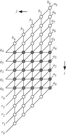
Detailed explanations of how a dependence graph could be obtained were presented in Chapters 10 and 11 and by the author elsewhere [86, 100, 116–118]. The dependence graph is two-dimensional (2-D) since we have two indices, i and j. If we consider only the gray circles, then the bounds on the indices are 0 ≤ i ≤ n − m = 4 and 0 ≤ j < m = 5. Each node in the algorithm performs the operations indicated in line 9 of Algorithm 18.1. If we extended the algorithm such that the inputs are fed from the same side and the outputs are obtained from the same side, then the bounds of the algorithm indices would be 0 ≤ i ≤ n + m and 0 ≤ j < m.
Coefficient qn−m−i of Q, on line 11 of Algorithm 18.1, is obtained at iteration i. Hence, this coefficient is represented by the ...
Get Algorithms and Parallel Computing now with the O’Reilly learning platform.
O’Reilly members experience books, live events, courses curated by job role, and more from O’Reilly and nearly 200 top publishers.

