8.5 DETECTING CYCLES IN THE ALGORITHM
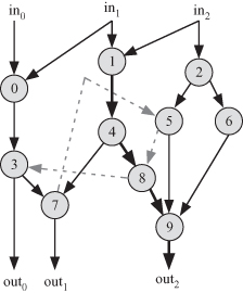
This section explains how cycles could be detected in the algorithm using the adjacency matrix A. Let us assume we modify the cycle-free algorithm in Fig. 8.1 to have an algorithm with a cycle in it like the one shown in Fig. 8.3. The dashed arrows indicate the extra links we added. Inspecting the figure indicates we have a cycle, 3 → 7 → 5 → 8 → 3.
Figure 8.3 Modifying the algorithm of Fig. 8.1 to contain a cycle as indicated by the dashed arrows.
The corresponding adjacency matrix is given by
(8.8)
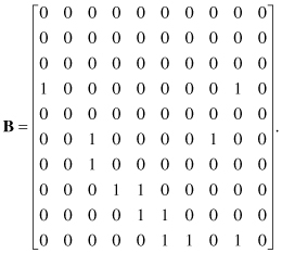
An inspection of the matrix would not reveal the presence of any cycle. In fact, nothing too interesting happens for powers of B2 and B3. However, for B4, the matrix takes on a very interesting form:
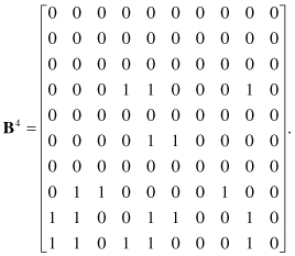
We note that there are four nonzero diagonal elements: b4 (3, 3), b4 (5, 5), b4 (7, 7), and b4 (8, 8). This indicates that there is a four-hop loop between nodes 3, 5, 7, and 8. The order of the loop can be determined by examining the rows associated with these nodes. Starting with node 3, we see that it depends on node 8. So, the path of the loop is 8 → 3. Now we look at row 8 and see that it depends on node 5. So, the path of the loop is ...
Get Algorithms and Parallel Computing now with the O’Reilly learning platform.
O’Reilly members experience books, live events, courses curated by job role, and more from O’Reilly and nearly 200 top publishers.

