Chapter 4. Collecting and Displaying Records
In this chapter, our first agile sprint, we climb level 1 of the data-value pyramid (Figure 4-1). We will connect, or plumb, the parts of our data pipeline all the way through from raw data to a web application on a user’s screen. This will enable a single developer to publish raw data records on the web. In doing so, we will activate our stack against our real data, thereby connecting our application to the reality of our data and our users.
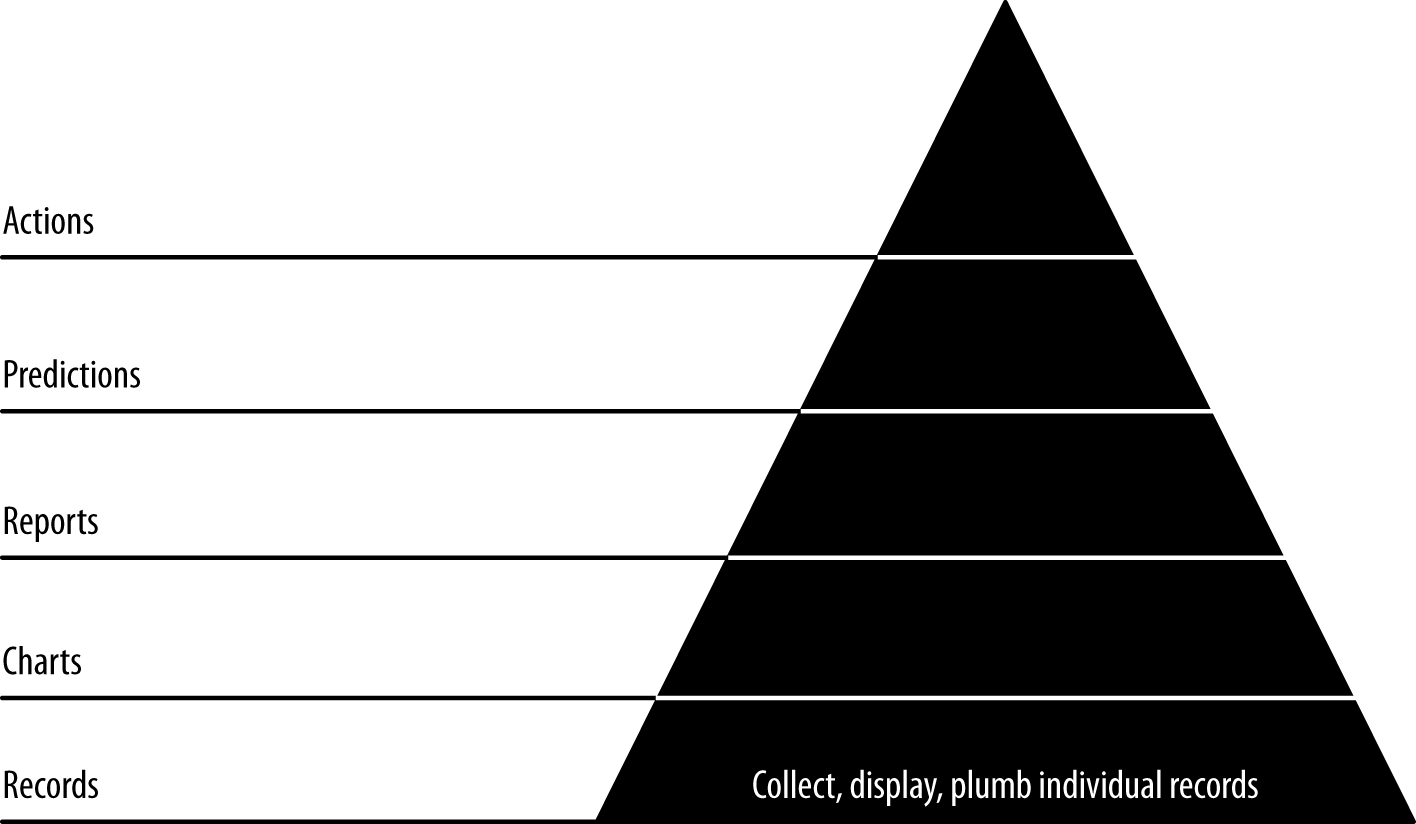
Figure 4-1. Level 1: displaying base records
If you already have a popular application, this step may seem confusing in that you already have the individual (or atomic) records displaying in your application. The point of this step, then, is to pipe these records through your analytical pipeline to bulk storage and then on to a browser. Bulk storage provides access for further processing via ETL (extract, transform, load) or some other means.
This first stage of the data-value pyramid can proceed relatively quickly, so we can get on to higher levels of value. Note that we will return to this step frequently as we enrich our analysis with additional datasets. We’ll make each new dataset explorable as we go. We’ll be doing this throughout the book as we work through the higher-level steps. The data-value pyramid is something you step up and down in as you do your analysis and get feedback from users. This setup and these browsable records set the stage for further advances up the data-value pyramid as our complexity and value snowball.
Note
If your atomic records are petabytes, you may not want to publish them all to a document store. Moreover, security constraints may make this impossible. In that case, a sample will do. Prepare a sample and publish it, and then constrain the rest of your application as you create it.
Code examples for this chapter are available at Agile_Data_Code_2/ch04. Clone the repository and follow along!
git clone https://github.com/rjurney/Agile_Data_Code_2.git
Putting It All Together
Setting up our stack was a bit of work. The good news is, with this stack, we don’t have to repeat this work as soon as we start to see load from users on our system increase and our stack needs to scale. Instead, we’ll be free to continue to iterate and improve our product from now on.
Now, let’s work with some atomic records—on-time records for each flight originating in the US in 2015—to see how the stack works for us.
Note
An atomic record is a base record, the most granular of the events you will be analyzing. We might aggregate, count, slice, and dice atomic records, but they are indivisible. As such, they represent ground truth to us, and working with atomic records is essential to plugging into the reality of our data and our application. The point of big data is to be able to analyze the most granular data using NoSQL tools to reach a deeper level of understanding than was previously possible.
Collecting and Serializing Flight Data
You can see the process of serializing events in Figure 4-2. In this case, we’re going to download the core data that we’ll use for the remainder of the book using a script, download.sh:
# Get on-time records for all flights in 2015 - 273MBwget -P data/\http://s3.amazonaws.com/agile_data_science/\On_Time_On_Time_Performance_2015.csv.bz2# Get openflights datawget -P /tmp/\https://raw.githubusercontent.com/jpatokal/openflights/\master/data/airports.dat mv /tmp/airports.dat data/airports.csv wget -P /tmp/\https://raw.githubusercontent.com/jpatokal/openflights/\master/data/airlines.dat mv /tmp/airlines.dat data/airlines.csv wget -P /tmp/\https://raw.githubusercontent.com/jpatokal/openflights/\master/data/routes.dat mv /tmp/routes.dat data/routes.csv wget -P /tmp/\https://raw.githubusercontent.com/jpatokal/openflights/\master/data/countries.dat mv /tmp/countries.dat data/countries.csv# Get FAA datawget -P data/ http://av-info.faa.gov/data/ACRef/tab/aircraft.txt wget -P data/ http://av-info.faa.gov/data/ACRef/tab/ata.txt wget -P data/ http://av-info.faa.gov/data/ACRef/tab/compt.txt wget -P data/ http://av-info.faa.gov/data/ACRef/tab/engine.txt wget -P data/ http://av-info.faa.gov/data/ACRef/tab/prop.txt
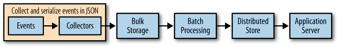
Figure 4-2. Serializing events
To get started, we’ll trim the unneeded fields from our on-time
flight records and convert them to Parquet format. This will improve
performance when loading this data, something we’ll be doing throughout
the book. In practice, you would want to retain all the values that might
be of interest in the future. Note that there is a bug in the
inferSchema option of spark-csv, so
we’ll have to cast the numeric fields manually before saving
our converted data.
If you want to make sense of the following query, take a look at the Bureau of Transportation Statistics description of the data, On-Time Performance records (this data was introduced in Chapter 3).
Run the following code to trim the data to just the fields we will need:
# Loads CSV with header parsing and type inference, in one line!on_time_dataframe=spark.read.format('com.databricks.spark.csv')\.options(header='true',treatEmptyValuesAsNulls='true',)\.load('data/On_Time_On_Time_Performance_2015.csv.bz2')on_time_dataframe.registerTempTable("on_time_performance")trimmed_cast_performance=spark.sql("""SELECTYear, Quarter, Month, DayofMonth, DayOfWeek, FlightDate,Carrier, TailNum, FlightNum,Origin, OriginCityName, OriginState,Dest, DestCityName, DestState,DepTime, cast(DepDelay as float), cast(DepDelayMinutes as int),cast(TaxiOut as float), cast(TaxiIn as float),WheelsOff, WheelsOn,ArrTime, cast(ArrDelay as float), cast(ArrDelayMinutes as float),cast(Cancelled as int), cast(Diverted as int),cast(ActualElapsedTime as float), cast(AirTime as float),cast(Flights as int), cast(Distance as float),cast(CarrierDelay as float), cast(WeatherDelay as float),cast(NASDelay as float),cast(SecurityDelay as float),cast(LateAircraftDelay as float),CRSDepTime, CRSArrTimeFROMon_time_performance""")# Replace on_time_performance table# with our new, trimmed table and show its contentstrimmed_cast_performance.registerTempTable("on_time_performance")trimmed_cast_performance.show()
Which shows a much simplified format (here abbreviated):
| Year | Quarter | Month | DayofMonth | DayOfWeek | FlightDate | Carrier | TailNum | FlightNum | Origin |
|---|---|---|---|---|---|---|---|---|---|
| 2015 | 1 | 1 | 1 | 4 | 2015-01-01 | AA | N001AA | 1519 | DFW |
| 2015 | 1 | 1 | 1 | 4 | 2015-01-01 | AA | N001AA | 1519 | MEM |
| 2015 | 1 | 1 | 1 | 4 | 2015-01-01 | AA | N002AA | 2349 | ORD |
| 2015 | 1 | 1 | 1 | 4 | 2015-01-01 | AA | N003AA | 1298 | DFW |
| 2015 | 1 | 1 | 1 | 4 | 2015-01-01 | AA | N003AA | 1422 | DFW |
Let’s make sure our numeric fields work as desired:
# Verify we can sum numeric columnsspark.sql("""SELECTSUM(WeatherDelay), SUM(CarrierDelay), SUM(NASDelay),SUM(SecurityDelay), SUM(LateAircraftDelay)FROM on_time_performance""").show()
This results in the following output (formatted to fit the page):
| sum(WeatherDelay) | sum(CarrierDelay) | sum(NASDelay) | sum(SecurityDelay) | sum(LateAircraftDelay) |
|---|---|---|---|---|
| 3100233.0 | 2.0172956E7 | 1.4335762E7 | 80985.0 | 2.4961931E7 |
Having trimmed and cast our fields and made sure the numeric columns work, we can now save our data as JSON Lines and Parquet. Note that we also load the data back, to verify that it loads correctly. Make sure this code runs without error, as the entire rest of the book uses these files:
# Save records as gzipped JSON Linestrimmed_cast_performance.toJSON()\.saveAsTextFile('data/on_time_performance.jsonl.gz','org.apache.hadoop.io.compress.GzipCodec')# View records on filesystem# gunzip -c data/On_Time_On_Time_Performance_2015.jsonl.gz/part-00000.gz | head# Save records using Parquettrimmed_cast_performance.write.parquet("data/on_time_performance.parquet")# Load JSON records backon_time_dataframe=spark.read.json('data/on_time_performance.jsonl.gz')on_time_dataframe.show()# Load the Parquet file backon_time_dataframe=spark.read.parquet('data/trimmed_cast_performance.parquet')on_time_dataframe.show()
Note that the Parquet file is only 248 MB, compared with 315 MB for the original gzip-compressed CSV and 259 MB for the gzip-compressed JSON. In practice the Parquet will be much more performant, as it will only load the individual columns we actually use in our PySpark scripts.
We can view the gzipped JSON with gunzip -c and
head:
gunzip -c data/On_Time_On_Time_Performance_2015.jsonl.gz/part-00000.gz | headWe can now view the on-time records directly, and understand them more easily than before:
{"Year":2015,"Quarter":1,"Month":1,"DayofMonth":1,"DayOfWeek":4,"FlightDate":"2015-01-01","UniqueCarrier":"AA","AirlineID":19805,"Carrier":"AA","TailNum":"N787AA","FlightNum":1,...}
Loading the gzipped JSON Lines data in PySpark is easy, using
a SparkSession called spark:
# Load JSON records back on_time_dataframe = spark.read.json('data/On_Time_On_Time_Performance_2015.jsonl.gz')on_time_dataframe.show()
Loading the Parquet data is similarly easy:
# Load the Parquet fileon_time_dataframe=spark.read.parquet('data/on_time_performance.parquet')on_time_dataframe.first()
Processing and Publishing Flight Records
Having collected our flight data, let’s process it (Figure 4-3). In the interest of plumbing our stack all the way through with real data to give us a base state to build from, let’s publish the on-time flight records right away to MongoDB and Elasticsearch, so we can access them from the web with Mongo, Elasticsearch, and Flask.
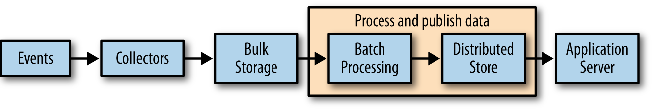
Figure 4-3. Processing and publishing data
Publishing Flight Records to MongoDB
MongoDB’s Spark integration makes this easy. We simply need to import and
activate pymongo_spark, convert our
DataFrame to an RDD, and call saveToMongoDB. We do this in ch04/pyspark_to_mongo.py:
importpymongoimportpymongo_spark# Important: activate pymongo_sparkpymongo_spark.activate()on_time_dataframe=spark.read.parquet('data/on_time_performance.parquet')# Note we have to convert the row to a dict# to avoid https://jira.mongodb.org/browse/HADOOP-276as_dict=on_time_dataframe.rdd.map(lambdarow:row.asDict())as_dict.saveToMongoDB('mongodb://localhost:27017/agile_data_science.on_time_performance')
If something goes wrong, you can always drop the collection and try again:
$mongoagile_data_science
> db.on_time_performance.drop()

true
The beauty of our infrastructure is that everything is reproducible from the original data, so there is little worrying to be done about our database becoming corrupted or crashing (although we do employ a fault-tolerant cluster). In addition, because we’re using our database as a document store, where we simply fetch documents by some ID or field, we don’t have to worry much about performance, either.
Finally, let’s verify that our flight records are in MongoDB:
> db.on_time_performance.findOne()

{
	"_id" : ObjectId("56f9ed67b0504718f584d03f"),
	"Origin" : "JFK",
	"Quarter" : 1,
	"FlightNum" : 1,
	"Div4TailNum" : "",
	"Div5TailNum" : "",
	"Div2TailNum" : "",
	"Div3TailNum" : "",
	"ArrDel15" : 0,
	"AirTime" : 378,
	"Div5WheelsOff" : "",
	"DepTimeBlk" : "0900-0959",
       ...
}
Now let’s fetch one flight record, using its minimum unique identifiers—the airline carrier, the flight date, and the flight number:
> db.on_time_performance.findOne(
  {Carrier: 'DL', FlightDate: '2015-01-01', FlightNum: 478})
You might notice that this query does not return quickly. Mongo lets us query our data by any combination of its fields, but there is a cost to this feature. We have to think about and maintain indexes for our queries. In this case, the access pattern is static, so the index is easy to define:
> db.on_time_performance.ensureIndex({Carrier: 1, FlightDate: 1, FlightNum: 1})This may take a few moments to run, but our queries will be fast thereafter. This is a small price to pay for the features Mongo gives us. In general, the more features of a database we use, the more we have to pay in terms of operational overhead. So, always try to use database features sparingly, unless you enjoy tuning databases in production.
Presenting Flight Records in a Browser
Now that we’ve published on-time flight records to a document store and queried them, we’re ready to present our data in a browser via a simple web application (Figure 4-4).
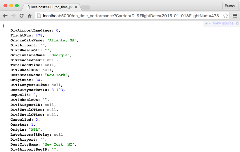
Figure 4-4. Displaying a raw flight record
Serving Flights with Flask and pymongo
Flask and pymongo make
querying and returning flights easy. ch04/web/on_time_flask.py
returns JSON about a flight on the web. This code might serve as an API,
and we’ll create and use JSON APIs later in the book. Note that we can’t
use json.dumps(), because we are
JSON-izing pymongo records, which
json doesn’t know how to serialize.
Instead we must use bson.json_util.dumps():
fromflaskimportFlask,render_template,requestfrompymongoimportMongoClientfrombsonimportjson_util# Set up Flask and Mongoapp=Flask(__name__)client=MongoClient()# Controller: Fetch a flight and display it@app.route("/on_time_performance")defon_time_performance():carrier=request.args.get('Carrier')flight_date=request.args.get('FlightDate')flight_num=request.args.get('FlightNum')flight=client.agile_data_science.on_time_performance.find_one({'Carrier':carrier,'FlightDate':flight_date,'FlightNum':flight_num})returnjson_util.dumps(flight)if__name__=="__main__":app.run(debug=True)
Rendering HTML5 with Jinja2
As we did in Chapter 3, let’s turn this raw JSON into a web page with a Jinja2 template. Check out ch04/web/on_time_flask_template.py. Jinja2 makes it easy to transform raw flight records into web pages:
fromflaskimportFlask,render_template,requestfrompymongoimportMongoClientfrombsonimportjson_util# Set up Flask and Mongoapp=Flask(__name__)client=MongoClient()# Controller: Fetch a flight and display it@app.route("/on_time_performance")defon_time_performance():carrier=request.args.get('Carrier')flight_date=request.args.get('FlightDate')flight_num=request.args.get('FlightNum')flight=client.agile_data_science.on_time_performance.find_one({'Carrier':carrier,'FlightDate':flight_date,'FlightNum':int(flight_num)})returnrender_template('flight.html',flight=flight)if__name__=="__main__":app.run(debug=True)
Note that render_template in our example points at the
file ch04/web/templates/flight.html.
This is a partial template that fills in the dynamic content area of our
layout page. The layout page that it subclasses, ch04/web/templates/layout.html,
imports Bootstrap and handles the global design for each page, such as
the header, overall styling, and footer. This saves us from repeating
ourselves in each page to create a consistent layout for the
application.
The layout template contains an empty content
block, {% block content %}{%
endblock %}, into which our partial template containing our
application data is rendered:
<!DOCTYPE html><htmllang="en"><head><metacharset="utf-8"><title>Agile Data Science</title><metaname="viewport"content="width=device-width, initial-scale=1.0"><metaname="description"content="Chapter 5 example in Agile Data Science, 2.0"><metaname="author"content="Russell Jurney"><linkhref="/static/bootstrap.min.css"rel="stylesheet"><linkhref="/static/bootstrap-theme.min.css"rel="stylesheet"></head><body><divid="wrap"><!--Begin page content--><divclass="container"><divclass="page-header"><h1>Agile Data Science</h1></div>{% block body %}{% endblock %}</div><divid="push"></div></div><divid="footer"><divclass="container"><pclass="muted credit"><ahref="http://shop.oreilly.com/product/ \ 0636920025054.do">\ Agile Data Science</a>by \<ahref="http://www.linkedin.com/in/ \ russelljurney">Russell Jurney</a>, 2016</div></div><scriptsrc="/static/bootstrap.min.js"></script></body></html>
Our flight-specific partial template works by
subclassing the layout template. Jinja2 templates perform control flow
in {% %} tags to loop through tuples
and arrays and apply conditionals. We display variables by putting bound
data or arbitrary Python code inside the {{ }} tags. For
example, our flight template looks like this:
{% extends "layout.html" %}
{% block body %}
  <div>
    <p class="lead">Flight {{flight.FlightNum}}</p>
    <table class="table">
      <thead>
        <th>Airline</th>
        <th>Origin</th>
        <th>Destination</th>
        <th>Tail Number</th>
        <th>Date</th>
        <th>Air Time</th>
        <th>Distance</th>
      </thead>
      <tbody>
        <tr>
          <td>{{flight.Carrier}}</td>
          <td>{{flight.Origin}}</td>
          <td>{{flight.Dest}}</td>
          <td>{{flight.TailNum}}</td>
          <td>{{flight.FlightDate}}</td>
          <td>{{flight.AirTime}}</td>
          <td>{{flight.Distance}}</td>
        </tr>
      </tbody>
    </table>
  </div>
{% endblock %}
Our body content block is what renders the page content for our data. We start with a raw template, plug in values from our data (via the flight variable we bound to the template), and get the page displaying a record.
We can see the flight in our web page with a
Carrier, FlightDate, and FlightNum. To test things out, grab a flight
record directly from MongoDB:
$mongoagile_data_science
>db.on_time_performance.findOne(){"_id":ObjectId("56fd7391b05047327f19241f"),"Origin":"IAH","FlightNum":1044,"Carrier":"AA","FlightDate":"2015-07-03","DivActualElapsedTime":null,"AirTime":122,"Div5WheelsOff":"","DestCityMarketID":32467,"Div3AirportID":null,"Div3TotalGTime":null,"Month":7,"CRSElapsedTime":151,"DestStateName":"Florida","DestAirportID":13303,"Distance":964,...}
We can now fetch a single flight via /ch04/web/templates/layout.html, as shown in Figure 4-5.
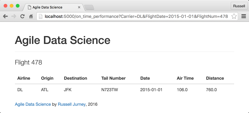
Figure 4-5. Presenting a single flight
Our Flask console shows the resources being accessed (dates and timestamps removed because of page width constraints):
127.0.0.1 - -[...]"GET /on_time_performance?Carrier=DL& \FlightDate=2015-01-01&FlightNum=478 HTTP/1.1"200- 127.0.0.1 - -[...]"GET /static/bootstrap.min.css HTTP/1.1"200- 127.0.0.1 - -[...]"GET /static/bootstrap-theme.min.css HTTP/1.1"200- 127.0.0.1 - -[...]"GET /static/bootstrap.min.js HTTP/1.1"200- 127.0.0.1 - -[...]"GET /favicon.ico HTTP/1.1"404-
Great! We made a web page from raw data! But ... so what? What have we achieved?
We’ve completed the base of the pyramid, level 1—displaying atomic records—in our standard data pipeline. This is a foundation. Whatever advanced analytics we offer, in the end, the user will often want to see the signal itself—that is, the raw data backing our inferences. There is no skipping steps here: if we can’t correctly “visualize” a single atomic record, then our platform and strategy have no base. They are weak.
Agile Checkpoint
Since we now have working software, it is time to let users in to start getting their feedback. “Wait, really? This thing is embarrassing!” Get over yourself!
We all want to be Steve Jobs; we all want to have a devastating product launch, and to make a huge splash with a top-secret invention. But with analytics applications, when you hesitate to ship, you let your fragile ego undermine your ability to become Steve Jobs by worrying about not looking like him in your first draft. If you don’t ship crap as step 1, you’re unlikely to get to a brilliant step 26. I strongly advise you to learn customer development and apply it to your projects. If you’re in a startup, the Startup Owner’s Manual by Steve Blank (K&S Ranch) is a great place to start.
You will notice immediately when you ship this
(maybe to close friends or insiders who clone the source from GitHub at
this point) that users can’t find which flights to retrieve by their
Carrier, FlightDate, and FlightNum. To get real utility from this data,
we need list and search capabilities.
You may well have anticipated this. Why ship something obviously broken or incomplete? Because although step 2 is obvious, step 13 is not. We must involve users at this step because their participation is a fundamental part of completing step 1 of the data-value pyramid. Users provide validation of our underlying assumptions, which at this stage might be stated in the form of two questions: “Does anyone care about flights?” and “What do they want to know about a given flight?” We think we have answers to these questions: “Yes” and “Airline, origin, destination, tail number, date, air time, and distance flown.” But without validation, we don’t really know anything for certain. Without user interaction and learning, we are building in the dark. Success that way is unlikely, just as a pyramid without a strong foundation will soon crumble.
The other reason to ship something now is that the act of publishing, presenting, and sharing your work will highlight a number of problems in your platform setup that would likely otherwise go undiscovered until the moment you launch your product. In Agile Data Science, you always ship after a sprint. As a team member, you don’t control whether to ship or not. You control what to ship and how broad an audience to release it to. This release might be appropriate for five friends and family members, and you might have to hound them to get it running or to click the link. But in sharing your budding application, you will optimize your packaging and resolve dependencies. You’ll have to make it presentable. Without such work, without a clear deliverable to guide your efforts, technical issues you are blinded to by familiarity will be transparent to you.
Now, let’s add listing flights and extend that to enable search, so we can start generating real clicks from real users.
Listing Flights
Flights are usually presented as a price-sorted list, filtered by the origin and destination, with the cheapest flight first. We lack price data, so instead we’ll list all flights on a given day between two destinations, sorted by departure time as a primary key, and arrival time as a secondary key. A list helps group individual flights with other similar flights. Lists are the next step in building this layer of the data-value pyramid, after displaying individual records.
Listing Flights with MongoDB
Before we search our flights, we need the capacity to list them in order to display our search results. We can use MongoDB’s query capabilities to return a list of flights between airports on a given day, sorted by departure and arrival time. The following queries are in ch04/mongo.js:
$mongoagile_data_science
> db.on_time_performance.find(
   {Origin: 'ATL', Dest: 'SFO', FlightDate: '2015-01-01'}).sort(
     {DepTime: 1, ArrTime: 1}) // Slow or broken
You may see this error:
error:{"$err":"too much data for sort() with no index. add an index or specify asmaller limit","code":10128}
If not, this query may still take a long time to complete, so let’s add another index for it. In general, we’ll need to add an index for each access pattern in our application, so always remember to do so up front in order to save yourself trouble with performance in the future:
> db.on_time_performance.ensureIndex({Origin: 1, Dest: 1, FlightDate: 1})Now that our index on origin, destination, and date is in place, we can get the flights between ATL and SFO on January 1, 2015:
>db.on_time_performance.find({Origin:'ATL',Dest:'SFO',FlightDate:'2015-01-01'}).sort({DepTime:1,ArrTime:1})// Fast
Our Flask stub works the same as before—except this time it passes an array of flights instead of one flight. This time, we’re using slugs in the URL for our web controller.1 A slug puts arguments in between forward slashes, instead of as query parameters. Check out this excerpt from ch04/web/on_time_flask_template.py:
# Controller: Fetch all flights between cities on a given day and display them@app.route("/flights/<origin>/<dest>/<flight_date>")deflist_flights(origin,dest,flight_date):flights=client.agile_data_science.on_time_performance.find({'Origin':origin,'Dest':dest,'FlightDate':flight_date},sort=[('DepTime',1),('ArrTime',1),])flight_count=flights.count()returnrender_template('flights.html',flights=flights,flight_date=flight_date,flight_count=flight_count)
Our templates are pretty simple too, owing to Bootstrap’s snazzy presentation of tables. Tables are often scoffed at by designers when used for layout, but this is tabular data, so their use is appropriate. To be extra snazzy, we’ve included the number of flights that day, and since the date is constant for all records, it is a field in the title of the page instead of a column:
{% extends "layout.html" %} {% block body %}<div><pclass="lead">{{flight_count}} Flights on {{flight_date}}</p><tableclass="table table-condensed table-striped"><thead><th>Airline</th><th>Flight Number</th><th>Origin</th><th>Destination</th><th>Departure Time</th><th>Tail Number</th><th>Air Time</th><th>Distance</th></thead><tbody>{% for flight in flights %}<tr><td>{{flight.Carrier}}</td><td><ahref="/on_time_performance?Carrier= {{flight.Carrier}}&FlightDate= {{flight.FlightDate}}&FlightNum= {{flight.FlightNum}}">{{flight.FlightNum}}</a></td><td>{{flight.Origin}}</td><td>{{flight.Dest}}</td><td>{{flight.DepTime}}</td><td>{{flight.TailNum}}</td><td>{{flight.AirTime}}</td><td>{{flight.Distance}}</td></tr>{% endfor %}</tbody></table></div>{% endblock %}
We can bind as many variables to a template as we want. Note that we also link from the list page (Figure 4-6) to the individual record pages, constructing the links out of the airline carrier, flight number, and flight date.
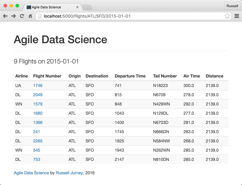
Figure 4-6. Presenting a list of flights
Paginating Data
Now that we can list the flights on a given day between cities, our users say, “What if I want to see lots of flights and there are so many on one page that it crashes my browser?” Listing hundreds of records is not a good presentation, and this will happen for other types of data. Shouldn’t there be a previous/next button to scroll forward and back in time? Yes. That is what we’ll add next.
So far we’ve glossed over how we’re creating these templates, subtemplates, and macros. Now we’re going to dive in by creating a macro and a subtemplate for pagination.
Reinventing the wheel?
Why are we building our own pagination? Isn’t that a solved problem?
The first answer is that it makes a good example to connect the browser with the data directly. In Agile Data Science, we try to process the data into the very state it takes on a user’s screen with minimal manipulation between the backend and an image in a browser. Why? We do this because it decreases complexity in our systems, because it unites data scientists and designers around the same vision, and because this philosophy embraces the nature of distributed systems in that it doesn’t rely on joins or other tricks that work best on “big iron,” or legacy systems.
Keeping the model consistent with the view is critical when the model is complex, as in a predictive system. We can best create value when the interaction design around a feature is cognizant of and consistent with the underlying data model. Data scientists must bring understanding of the data to the rest of the team, or the team can’t build to a common vision. The principle of building a view to match the model ensures this from the beginning.
In practice, we cannot predict at which layer a feature will arise. It may first appear as a burst of creativity from a web developer, designer, data scientist, or platform engineer. To validate it, we must ship it in an experiment as quickly as possible, and so the implementation layer of a feature may in fact begin at any level of our stack. When this happens, we must take note and ticket the feature as containing technical debt. As the feature stabilizes, if it is to remain in the system, we move it further back in the stack as time permits.
A full-blown application framework like Rails or Django would likely build in this functionality. However, when we are building an application around derived data, the mechanics of interactions often vary in both subtle and dramatic ways. Most web frameworks are optimized around CRUD operations. In big data exploration and visualization, we’re only doing the read part of CRUD, and we’re doing relatively complex visualization as part of it. Frameworks offer less value in this situation, where their behavior must likely be customized. Also note that while MongoDB happens to include the ability to select and return a range of sorted records, the NoSQL store you use may or may not provide this functionality, or it may not be possible to use this feature because publishing your data in a timely manner requires a custom service. You may have to precompute the data periodically and serve the list yourself. NoSQL gives us options, and web frameworks are optimized for relational databases. We must often take matters into our own hands.
Serving paginated data
To start, we’ll need to change our controller for flights to use
pagination
via MongoDB. There is a little math to do, since MongoDB
pagination uses skip and limit instead of start
and end. We need to compute the width of the query
by subtracting the start from the end, then applying this width in a
limit call:
# Controller: Fetch all flights between cities on a given day and display them@app.route("/flights/<origin>/<dest>/<flight_date>")deflist_flights(origin,dest,flight_date):start=request.args.get('start')or0start=max(int(start)-1,0)end=request.args.get('end')or20end=int(end)width=end-startflights=client.agile_data_science.on_time_performance.find({'Origin':origin,'Dest':dest,'FlightDate':flight_date},sort=[('DepTime',1),('ArrTime',1),]).skip(start).limit(width)flight_count=flights.count()returnrender_template('flights.html',flights=flights,flight_date=flight_date,flight_count=flight_count)
Prototyping back from HTML
In order to implement pagination in our templates, we need to prototype back from HTML. We’re all familiar with next/previous buttons from browsing flights on airline websites. We’ll need to set up the same thing for listing flights. We need links at the bottom of the flight list page (Figure 4-7) that allow you to paginate forward and back.

Figure 4-7. Missing next/previous links
More specifically, we need a link to an incremented/decremented offset range for the path /flights/<origin>/<dest>/<date>?start=N&end=N. Let’s prototype the feature based on these requirements by appending static forward and back links against our flight list API (Figure 4-8).
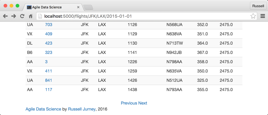
Figure 4-8. Simple next/previous links
For example, we want to dynamically render this HTML, corresponding to the URL /flights/JFK/LAX/2015-01-01?start=20&end=40:
# /ch04/templates/partials/flights.html ...<divstyle="text-align: center"><ahref="/flights/{{origin}}/{{dest}}/{{flight_date}}?start=0&end=20">Previous</a><ahref="/flights/{{origin}}/{{dest}}/{{flight_date}}?start=20&end=40">Next</a></div>{% endblock -%}
Pasting and navigating to the links, such as http://localhost:5000/flights/JFK/LAX/2015-01-01?start=20&end=40, demonstrates that the feature works with our data.
Now let’s generalize it. Macros are convenient, but we don’t want to make our template too complicated, so we compute the increments in a Python helper (we might consider a model class) and make a macro to render the offsets.
For starters, let’s use this opportunity to set up a simple config file to set variables like the number of records to display per page (embedding these in code will cause headaches later):
# ch04/web/config.py, a configuration file for index.pyRECORDS_PER_PAGE=20
Let’s also create a simple helper to calculate record offsets. In time this will become a full-blown class model, but for now, we’ll just create a couple of helper methods in /ch04/web/on_time_flask_template.py:
# Process Elasticsearch hits and return flight recordsdefprocess_search(results):records=[]ifresults['hits']andresults['hits']['hits']:total=results['hits']['total']hits=results['hits']['hits']forhitinhits:record=hit['_source']records.append(record)returnrecords,total# Calculate offsets for fetching lists of flights from MongoDBdefget_navigation_offsets(offset1,offset2,increment):offsets={}offsets['Next']={'top_offset':offset2+increment,'bottom_offset':offset1+increment}offsets['Previous']={'top_offset':max(offset2-increment,0),'bottom_offset':max(offset1-increment,0)}# Don't go < 0returnoffsets# Strip the existing start and end parameters from the query stringdefstrip_place(url):try:p=re.match('(.+)&start=.+&end=.+',url).group(1)exceptAttributeError,e:returnurlreturnp
The controller now employs the helper to generate and then bind the navigation variables to the template, because we are now passing both the list of flights and the calculated offsets for the navigation links. Check out ch04/web/on_time_flask_template.py:
# Controller: Fetch all flights between cities on a given day and display them@app.route("/flights/<origin>/<dest>/<flight_date>")deflist_flights(origin,dest,flight_date):start=request.args.get('start')or0start=int(start)end=request.args.get('end')or20end=int(end)width=end-startnav_offsets=get_navigation_offsets(start,end,config.RECORDS_PER_PAGE)flights=client.agile_data_science.on_time_performance.find({'Origin':origin,'Dest':dest,'FlightDate':flight_date},sort=[('DepTime',1),('ArrTime',1),])flight_count=flights.count()flights=flights.skip(start).limit(width)returnrender_template('flights.html',flights=flights,flight_date=flight_date,flight_count=flight_count,nav_path=request.path,nav_offsets=nav_offsets)
Our flight list template, ch04/web/templates/flights.html,
calls a macro to render our data. Note the use of |safe to ensure our HTML isn’t
escaped:
  {% import "macros.jnj" as common %}
  {% if nav_offsets and nav_path -%}
    {{ common.display_nav(nav_offsets, nav_path, flight_count, query)|safe }}
  {% endif -%}
We place this in our Jinja2 macros file,
further breaking up the task as the drawing of two links inside a
div:
ch04/web/templates/macros.jnj<!-- Display two navigation links for previous/next page in the flight list -->{% macro display_nav(offsets, path, count, query) -%}<divstyle="text-align: center;">{% for key, values in offsets.items() -%} {%- if values['bottom_offset'] >= 0 and values['top_offset'] > 0 and count > values['bottom_offset'] -%}<astyle="margin-left: 20px; margin-right: 20px;"href="{{ path }}?start={{ values['bottom_offset'] }}&end={{ values['top_offset']}}{%- if query -%}?search={{query}}{%- endif -%}">{{ key }}</a>{% else -%} {{ key }} {% endif %} {% endfor -%}</div>{% endmacro -%}
And we’re done. We can now paginate through our list of flights as we would in any other flight website. We’re one step closer to providing the kind of user experience that will enable real user sessions, and we’ve extended a graph connecting flights over the top of our individual records. This additional structure will enable even more structure later on, as we climb the data-value pyramid.
Searching for Flights
Browsing through a list of flights certainly beats manually looking
up message_ids, but it’s hardly as
efficient as searching for flights of interest. Let’s use our data
platform to add search.
Creating Our Index
Before we can store our documents in Elasticsearch, we need to create a search index for them to reside in. Check out elastic_scripts/create.sh. Note that we create only a single shard with a single replica. In production, you would want to distribute the workload around a cluster of multiple machines with multiple shards, and to achieve redundancy and high availability with multiple replicas of each shard. For our purposes, one of each is fine!
#!/usr/bin/env bashcurl -XPUT'http://localhost:9200/agile_data_science/'-d'{"settings" : {"index" : {"number_of_shards" : 1,"number_of_replicas" : 1}}}'
Go ahead and run the script, before we move on to publishing our on-time performance records to Elasticsearch:
elastic_scripts/create.sh
Note that if you want to start over, you can blow away the
agile_data_science index with:
elastic_scripts/drop.sh
And just like the create script, it calls
curl:
#!/usr/bin/env bashcurl -XDELETE'http://localhost:9200/agile_data_science/'
Publishing Flights to Elasticsearch
Using the recipe we created in Chapter 2, it is easy to publish our on-time performance flight data to Elasticsearch. Check out ch04/pyspark_to_elasticsearch.py:
# Load the Parquet fileon_time_dataframe=spark.read.parquet('data/on_time_performance.parquet')# Save the DataFrame to Elasticsearchon_time_dataframe.write.format("org.elasticsearch.spark.sql")\.option("es.resource","agile_data_science/on_time_performance")\.option("es.batch.size.entries","100")\.mode("overwrite")\.save()
Note that we need to set es.batch.size.entries to
100, down from the default of
1000. This keeps Elasticsearch from being overwhelmed
by Spark. You can find other settings to adjust in the configuration guide.
Note that this might take some time, as there are several million records to index. You might want to leave this alone to run for a while. You can interrupt it midway and move on; so long as some records are indexed you should be okay. Similarly, if there is an error, you should check the results of the following query; it might be possible to disregard the error and just move on, if enough records have been indexed for the rest of the examples.
Querying our data with curl is easy. This time,
let’s look for flights originating in Atlanta (airport code ATL), the
world’s busiest airport:
curl\'localhost:9200/agile_data_science/on_time_performance/ \_search?q=Origin:ATL&pretty'
The output looks like so:
{"took":7,"timed_out":false,"_shards":{"total":5,"successful":5,"failed":0},"hits":{"total":379424,"max_score":3.7330098,"hits":[{"_index":"agile_data_science","_type":"on_time_performance","_id":"AVakkdOGX8o-akD569e2","_score":3.7330098,"_source":{"Year":2015,"Quarter":3,"Month":9,"DayofMonth":23,"DayOfWeek":3,"FlightDate":"2015-09-23","UniqueCarrier":"DL",...
Note the useful information our query returned along with the records found: how long the query took (7 ms) and the total number of records that matched our query (379,424).
Searching Flights on the Web
Next, let’s connect our search engine to the web.
First, configure pyelastic
to point at our Elasticsearch server:
# ch04/web/config.pyELASTIC_URL='http://localhost:9200/agile_data_science'
Then import, set up, and query Elasticsearch via the /flights/search path in ch04/web/on_time_flask_template.py:
@app.route("/flights/search")defsearch_flights():# Search parameterscarrier=request.args.get('Carrier')flight_date=request.args.get('FlightDate')origin=request.args.get('Origin')dest=request.args.get('Dest')tail_number=request.args.get('TailNum')flight_number=request.args.get('FlightNum')# Pagination parametersstart=request.args.get('start')or0start=int(start)end=request.args.get('end')orconfig.RECORDS_PER_PAGEend=int(end)nav_offsets=get_navigation_offsets(start,end,config.RECORDS_PER_PAGE)# Build our Elasticsearch queryquery={'query':{'bool':{'must':[]}},'sort':[{'FlightDate':{'order':'asc','ignore_unmapped':True}},{'DepTime':{'order':'asc','ignore_unmapped':True}},{'Carrier':{'order':'asc','ignore_unmapped':True}},{'FlightNum':{'order':'asc','ignore_unmapped':True}},'_score'],'from':start,'size':config.RECORDS_PER_PAGE}ifcarrier:query['query']['bool']['must'].append({'match':{'Carrier':carrier}})ifflight_date:query['query']['bool']['must'].append({'match':{'FlightDate':flight_date}})iforigin:query['query']['bool']['must'].append({'match':{'Origin':origin}})ifdest:query['query']['bool']['must'].append({'match':{'Dest':dest}})iftail_number:query['query']['bool']['must'].append({'match':{'TailNum':tail_number}})ifflight_number:query['query']['bool']['must'].append(\n||||{...}\n||||)# where |# is a spaceresults=elastic.search(query)flights,flight_count=process_search(results)# Persist search parameters in the form templatereturnrender_template('search.html',flights=flights,flight_date=flight_date,flight_count=flight_count,nav_path=request.path,nav_offsets=nav_offsets,carrier=carrier,origin=origin,dest=dest,tail_number=tail_number,flight_number=flight_number)
Generalizing the navigation links, we are able to use a similar template for searching flights as we did for listing them. We’ll need a form to search for flights against specific fields, so we create one at the top of the page. We have parameterized the template with all of our search arguments, to persist them through multiple submissions of the form. Check out ch04/web/templates/search.html:
<formaction="/flights/search"method="get"><labelfor="Carrier">Carrier</label><inputname="Carrier"maxlength="3"style="width: 40px; margin-right: 10px;"value="{{carrier}}"></input><labelfor="Origin">Origin</label><inputname="Origin"maxlength="3"style="width: 40px; margin-right: 10px;"value="{{origin}}"></input><labelfor="Dest">Dest</label><inputname="Dest"maxlength="3"style="width: 40px; margin-right: 10px;"value="{{dest}}"></input><labelfor="FlightDate">FlightDate</label><inputname="FlightDate"style="width: 100px; margin-right: 10px;"value="{{flight_date}}"></input><labelfor="TailNum">TailNum</label><inputname="TailNum"style="width: 100px; margin-right: 10px;"value="{{tail_number}}"></input><labelfor="FlightNum">FlightNum</label><inputname="FlightNum"style="width: 50px; margin-right: 10px;"value="{{flight_number}}"></input><buttontype="submit"class="btn btn-xs btn-default"style="height: 25px">Submit</button></form>
Figure 4-9 shows the result.
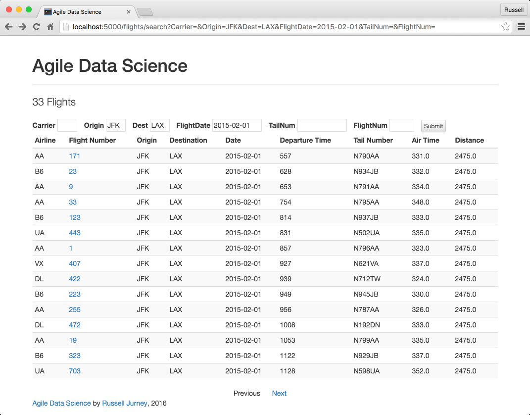
Figure 4-9. Searching for flights
Conclusion
We have now collected, published, indexed, displayed, listed, and searched flight records. They are no longer abstract. We can search for flights, click on individual flights, and explore as we might any other dataset. More importantly, we have piped our raw data through our platform and transformed it into an interactive application.
This application forms the base of our value stack. We will use it as the way to develop, present, and iterate on more advanced features throughout the book as we build value while walking up the data-value pyramid. With the base of the pyramid in place, we can move on to building charts.
1 For more on controllers, see Alex Coleman’s blog post on MVC in Flask.
Get Agile Data Science 2.0 now with the O’Reilly learning platform.
O’Reilly members experience books, live events, courses curated by job role, and more from O’Reilly and nearly 200 top publishers.

