CHAPTER 19ERROR ELLIPSE
19.1 INTRODUCTION
![]() As discussed previously, after completing a least squares adjustment, the estimated standard deviations in the coordinates of an adjusted station can be calculated from covariance matrix elements. These standard deviations provide error estimates in the reference axes directions. In graphical representation, they are half the dimensions of a standard error rectangle centered on each station. The standard error rectangle has dimensions of 2Sx by 2Sy as illustrated for station B in Figure 19.1, but this is not a true representation of the error present at the station.
As discussed previously, after completing a least squares adjustment, the estimated standard deviations in the coordinates of an adjusted station can be calculated from covariance matrix elements. These standard deviations provide error estimates in the reference axes directions. In graphical representation, they are half the dimensions of a standard error rectangle centered on each station. The standard error rectangle has dimensions of 2Sx by 2Sy as illustrated for station B in Figure 19.1, but this is not a true representation of the error present at the station.
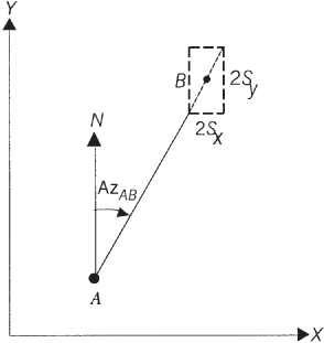
FIGURE 19.1 Standard error rectangle.
Simple deductive reasoning can be used to show the basic problem. Assume in Figure 19.1 that the XY coordinates of station A have been computed from the observations of distance AB and azimuth AzAB, which is approximately 30°. Further assume that the observed azimuth has no error at all, but that the distance has a large error, say ±2 ft. From Figure 19.1, it should then be readily apparent that the largest uncertainty in the station's position would not lie in either cardinal direction. That is, neither Sx nor Sy represents the largest positional uncertainty for the station. Rather, the largest uncertainty would be collinear with line ...
Get Adjustment Computations, 6th Edition now with the O’Reilly learning platform.
O’Reilly members experience books, live events, courses curated by job role, and more from O’Reilly and nearly 200 top publishers.

