Chapter 1. An Introduction to Performance Tuning
There are a thousand hacking at the branches of evil to one who is striking at the root.
Going faster seems to be a central part of human development. As little as three hundred years ago, the fastest you could expect to go was a few tens of miles an hour, aboard a fast clipper ship with a stiff wind behind you. Now, we must expand our view to things such as the fastest achievable speed while remaining in the Earth’s atmosphere -- perhaps fifteen hundred miles an hour, twice the speed of sound, if you are a civilian without access to the latest, fastest military aircraft. The journey that used to take three weeks under sail from London to New York City now takes us as little as two and a half hours, sipping champagne the whole way.
This innate human desire to go fast is expressed in many ways: microwave ovens let us cook dinner quickly, high-performance automobiles and motorcycles give us a wonderful thrill, email lets us communicate at almost the speed of thought. But what happens when that email server is overwhelmed, as when we all log in at eight o’clock in the morning to check what has gone on while we’ve slept? Or when the procurement system for the company that distributes microwave ovens is only able to handle half of the workload, or when a mechanical engineer’s CAD system runs so slowly that the car engine she’s designing won’t be ready in time for the new model year?
These are the problems facing us in performance tuning: it is the adaptation of the speed of a computer system to the speed requirements imposed by the real world.
Sometimes these problems are subtle, sometimes not. We must carefully consider the changes in the system that caused it to become unacceptably slow. These influences might come from within, such as a heavier load placed on the system, or from without, such as a new operating system revision subtly changing -- or utterly replacing -- an algorithm for resource management that is critically important to our software. The solutions are sometimes quick (a matter of adjusting one “knob” slightly), or sometimes slow and painful (a task for weeks of analysis, consultations with vendors, and careful redesign of an infrastructure).
When I originally started work on this book, it seemed straightforward: take Mike Loukides’s excellent but dated first edition and overhaul it for modern computer systems. As I progressed further along, I realized that this book is actually about much more than simply performance tuning. It really covers two distinct areas:
These areas are all underpinned by the science of computer architecture. This book does not concentrate on application design; rather, it focuses on the operating system, the underlying hardware, and their interactions.
To most systems administrators, a computer is really a black box. This is perfectly reasonable for many tasks: after all, it’s certainly not necessary to understand how the operating system manages free memory to configure and maintain a mail server. However, in performance tuning -- which is, at heart, very much about the underlying hardware and how it is abstracted -- truly understanding the behavior of the system involves a detailed knowledge of the inner workings of the machine. In this chapter, we’ll briefly discuss some of the most important concepts of computer architecture, and then go into the fundamental principles of performance tuning.
An Introduction to Computer Architecture
A full discussion of computer architecture is far beyond the level of this text. Periodically, we’ll go into architectural matters, in order to provide the conceptual underpinnings of the system under discussion. However, if this sort of thing interests you, there are a great many excellent texts on the topic. Perhaps the most commonly used are two textbooks by John Hennessy and David Patterson: they are titled Computer Organization and Design: The Hardware/Software Interface and Computer Architecture: A Quantitative Approach (both published by Morgan Kaufmann).
In this section, we’ll focus on the two most important general concepts of architecture: the general means by which we approach a problem (the levels of transformation), and the essential model around which computers are designed.
Levels of Transformation
When we approach a problem, we must reduce it to something that a computer can understand and work with: this might be anything from a set of logic gates, solving the fundamental problem of “How do we build a general-purpose computing machine?” to a few million bits worth of binary code. As we proceed through these logical steps, we transform the problem into a “simpler” one (at least from the computer’s point of view). These steps are the levels of transformation.
Software: algorithms and languages
When faced with a problem where we think a computer will be of assistance, we first develop an algorithm for completing the task in question. Algorithms are, very simply, a repetitive set of instructions for performing a particular task -- for example, a clerk inspecting and routing incoming mail follows an algorithm for how to properly sort the mail.
This algorithm must then be translated by a programmer into a program written in a language.[1] Generally, this is a high-level language, such as C or Perl, although it might be a low-level language, such as assembler. The language layer exists to make our lives easier: the structure and grammar of high-level languages lets us easily write complex programs. This high-level language program, which is usually portable between different systems, is then transformed by a compiler into the low-level instructions required by a specific system. These instructions are specified by the Instruction Set Architecture.
The Instruction Set Architecture
The Instruction Set Architecture, or ISA, is the fundamental language of the microprocessor: it defines the basic, indivisible instructions that we can execute. The ISA serves as the interface between software and hardware. Examples of instruction set architectures include IA-32, which is used by Intel and AMD CPUs; MIPS, which is implemented in the Silicon Graphics/MIPS R-series microprocessors (e.g., the R12000); and the SPARC V9 instruction set used by the Sun Microsystems UltraSPARC series.
Hardware: microarchitecture, circuits, and devices
At this level, we are firmly in the grasp of electrical and computer engineering. We concern ourselves with functional units of microarchitecture and the efficiency of our design. Below the microarchitectural level, we worry about how to implement the functional units through circuit design: the problems of electrical interference become very real. A full discussion of the hardware layer is far beyond us here; tuning the implementations of microprocessors is not something we are generally able to do.
The von Neumann Model
The von Neumann model has served as the basic design model for all modern computing systems: it provides a framework upon which we can hang the abstractions and flesh generated by the levels of transformation.[2] The model consists of four core components:
A memory system, which stores both instructions and data. This is known as a stored program computer. This memory is accessed by means of the memory address register (MAR), where the system puts the address of a location in memory, and a memory data register (MDR), where the memory subsystem puts the data stored at the requested location. I discuss memory in more detail in Chapter 4.
At least one processing unit, often known as the arithmetic and logic unit (ALU). The processing units are more commonly called the central processing unit (CPU).[3] It is responsible for the execution of all instructions. The processor also has a small amount of very fast storage space, called the register file. I discuss processors in detail in Chapter 3.
A control unit, which is responsible for controlling cross-component operations. It maintains a program counter, which contains the next instruction to be loaded, and an instruction register, which contains the current instruction. The peculiarities of control design are beyond the scope of this text.
The system needs a nonvolatile way to store data, as well as ways to represent it to the user and to accept input. This is the domain of the input/output (I/O) subsystem. This book primarily concerns itself with disk drives as a mechanism for I/O; I discuss them in Chapter 5. I also discuss network I/O in Chapter 7.
Despite all the advances in computing over the last sixty years, they all fit into this framework. That is a very powerful statement: despite the fact that computers are orders of magnitude faster now, and being used in ways that weren’t even imaginable at the end of the Second World War, the basic ideas, as formulated by von Neumann and his colleagues, are still applicable today.
Caches and the Memory Hierarchy
As you’ll see in Section 1.2 later in this chapter, one of the principles of performance tuning is that there are always trade-offs. This problem was recognized by the pioneers in the field, and we still do not have a perfect solution today. In the case of data storage, we are often presented with the choice between cost, speed, and size. (Physical parameters, such as heat dissipation, also play a role, but for this discussion, they’re usually subsumed into the other variables.) It is possible to build extremely large, extremely fast memory systems -- for example, the Cray 1S supercomputer used very fast static RAM exclusively for memory.[4] This is not something that can be adapted across the spectrum of computing devices.
The problem we are trying to solve is that storage size tends to be inversely proportional to performance, particularly relative to the next highest level of price/performance. A modern microprocessor might have a cycle time measured in fractions of a nanosecond, while making the trip to main memory can easily be fifty times slower.
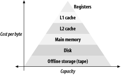
To try and work around this problem, we employ something known as the memory hierarchy. It is based on creating a tree of storage areas (Figure 1-1). At the top of the pyramid, we have very small areas of storage that are exceedingly fast. As we progress down the pyramid, things become increasingly slow, but correspondingly larger. At the foundation of the pyramid, we might have storage in a tape library: many terabytes, but it might take minutes to access the information we are looking for.
Tip
From the point of view of the microprocessor, main memory is very slow. Anything that makes us go to main memory is bad -- unless we’re going to main memory to prevent going to an even slower storage medium (such as disk).
The function of the pyramid is to cache the most frequently used data and instructions in the higher levels. For example, if we keep accessing the same file on tape, we might want to store a temporary copy on the next fastest level of storage (disk). We can similarly store a file we keep accessing from disk in main memory, taking advantage of main memory’s substantial performance benefit over disk.
The Benefits of a 64-Bit Architecture
Companies that produced computer hardware and software often make a point of mentioning the size of their systems’ address space (typically 32 or 64 bits). In the last five years, the shift from 32-bit to 64-bit microprocessors and operating systems has caused a great deal of hype to be generated by various marketing departments. The truth is that although in certain cases 64-bit architectures run significantly faster than 32-bit architectures, in general, performance is equivalent.
What does it mean to be 64-bit?
The number of “bits” refers to the width of a data path. However, what this actually means is subject to its context. For example, we might refer to a 16-bit data path (for example, UltraSCSI). This means that the interconnect can transfer 16 bits of information at a time. With all other things held constant, it would be twice as fast as an interconnect with a 8-bit data path.
The “bitness” of a memory system refers to how many wires are used to transfer a memory address. For example, if we had an 8-bit path to the memory address, and we wanted the 19th location in memory, we would turn on the appropriate wires (1, 2, and 5; we derive this from writing 19 in binary, which gives 00010011 -- everywhere there is a one, we turn on that wire). Note, however, that since we only have 8 bits worth of addressing, we are limited to 64 (28) addresses in memory. 32-bit systems are, therefore, limited to 4,294,967,296 (232) locations in memory. Since memory is typically accessible in 1-byte blocks, this means that the system can’t directly access more than 4 GB of memory. The shift to 64-bit operating systems and hardware means that the maximum amount of addressable memory is about 16 petabytes (16777216 GB), which is probably sufficient for the immediately forseeable future.
Unfortunately, it’s often not quite this simple in practice. A 32-bit SPARC system is actually capable of having more than 4 GB of memory installed, but, in Solaris, no single process can use more than 4 GB. This is because the hardware that controls memory management actually uses a 44-bit addressing scheme, but the Solaris operating system can only give any one process the amount of memory addressable in 32 bits.
Performance ramifications
The change from 32-bit to 64-bit architectures, then, expanded the size of main memory and the amount of memory a single process can have. An obvious question is, how did applications benefit from this? Here are some kinds of applications that benefitted from larger memory spaces:
Applications that could not use the most time-efficient algorithm for a problem because that algorithm would use more than 4 GB of memory.
Applications where caching large data sets is critically important, and therefore the more memory available to the process, the more can be cached.
Applications where the system is short on memory due to overwhelming utilization (many small processes). Note that in SPARC systems, this was not a problem: each process could only see 4 GB, but the system could have much more installed.
In general, the biggest winners from 64-bit systems are high-performance computing and corporate database engines. For the average desktop workstation, 32 bits is plenty.
Unfortunately, the change to 64-bit systems also meant that the underlying operating system and system calls needed to be modified, which sometimes resulted in a slight slowdown (for example, more data needs to be manipulated during pointer operations). This means that there may be a very slight performance penalty associated with running in 64-bit mode.
Principles of Performance Tuning
In this book, I present a few “rules of thumb.” As an old IBM technical bulletin says, rules of thumb come from people who live out of town and who have no production experience.[5]
Keeping that in mind, I’ve found that much of the conceptual basis behind system performance tuning can be summarized in five principles: understand your environment, nothing is ever free, throughput and latency are distinct measurements, resources should not be overutilized, and one must design experiments carefully.
Principle 0: Understand Your Environment
If you don’t understand your environment, you can’t possibly fix the problem. This is why there is such an emphasis on conceptual material throughout this text: even though the specific details of how an algorithm is implemented might change, or even the algorithm itself, the abstract knowledge of what the problem is and how it is approached is still valid. You have a much more powerful tool at your disposal if you understand the problem than if you know a solution without understanding why the problem exists.
Certainly, at some level, problems are well beyond the scope of the average systems administrator: tuning network performance at the level discussed here does not really require an in-depth understanding of how the TCP/IP stack is implemented in terms of modules and function calls. If you are interested in the inner details of how the different variants of the Unix operating system work, there are a few excellent texts that I strongly suggest you read: Solaris Kernel Internals by Richard McDougall and James Mauro, The Design of the UNIX Operating System by Maurice J. Bach, and Operating Systems, Design and Implementation by Andrew Tanenbaum and Andrew Woodfull (all published by Prentice Hall).
The ultimate reference, of course, is the source code itself. As of this writing, the source code for all the operating systems I describe in detail (Solaris and Linux) is available for free.
Principle 1: TANSTAAFL!
TANSTAAFL means There Ain’t No Such Thing As A Free Lunch.[6] At heart, performance tuning is about making trade-offs between various attributes. This usually consists of a list of three desirable attributes -- of which we can pick only two.
One example comes from tuning the TCP network layer, where Nagle’s algorithm provides a way to sacrifice latency, or the time required to deliver a single packet, in exchange for increased throughput, or how much data can be effectively pushed down the wire. (We’ll discuss Nagle’s algorithm in greater detail in Section 7.4.2.8.)
This principle often necessitates making real, significant, and difficult choices.
Principle 2: Throughput Versus Latency
In many ways, systems administrators who are evaluating computer systems are often like adolescent males evaluating cars. This is unfortunate. In both cases, there are a certain set of metrics, and we try to find the highest value for the most “important” metric. Typically, these are “bulk data throughput” for computers and “horsepower” for cars.
The lengths to which some people will go to obtain maximum horsepower from their four-wheeled vehicles are often somewhat ludicrous. A slight change in perspective would reveal that there are other facets to the performance gem. A lot of effort is spent in optimizing a single thing that may not actually be a problem. I would like to illustrate this by means of a simplistic comparison (please remember that we are comparing performance alone). Vehicle A puts out about 250 horsepower, whereas Vehicle B only produces about 95. One would assume that Vehicle A exhibits significantly “better” performance in the real world than Vehicle B. The astute reader may ask what the weights of the vehicles involved are: Vehicle A weighs about 3600 pounds, whereas Vehicle B weighs about 450. It is then apparent that Vehicle B is actually quite a bit faster (0-60 mph in about three and a half seconds, as opposed to Vehicle A’s leisurely five and a half seconds). However, when we compare how fast the vehicles actually travel in crowded traffic down Highway 101 (which runs down the San Francisco Peninsula), Vehicle B wins by an even wider margin, since motorcycles in California are allowed to ride between the lanes (“lane splitting”).[7]
Perhaps the most often neglected consideration in this world of tradeoffs is latency. For example, let’s consider a fictional email server application -- call it SuperDuperMail. The SuperDuperMail marketing documentation claims that it is capable of handling over one million messages a hour. This might seem pretty reasonable: this rate is far faster than most companies need. In other words, the throughput is generally good. A different way of looking at the performance of this mail server would be to ask how long it takes to process a single message. After some pointed questions to the SuperDuperMail marketing department, they reveal that it takes half an hour to process a message. This appears contradictory: it would seem to indicate that the software can process at most two messages an hour. However, it turns out that the SuperDuperMail product is based on a series of bins internally, and moves messages to the next bin only when that bin is completely full. In this example, despite the fact that throughput is acceptable, the latency is horrible. Who wants to send a message to the person two offices down and have it take half an hour to get there?
Principle 3: Do Not Overutilize a Resource
Anyone who has driven on a heavily-travelled highway has seen a very common problem in computing emerge in a different area: the “minimum speed limit” signs often seem like a cruel joke! Clearly, there are many factors that go into designing and maintaining an interstate, particularly one that is heavily used by commuters: the peak traffic is significantly different than the average traffic, funding is always a problem, etc. Furthermore, adding another lane to the highway, assuming that space and funding is available, usually involves temporarily closing at least one lane of the active roadway. This invariably frustrates commuters even more. The drive to provide “sufficient” capacity is always there, but the barriers to implementing change are such that it often takes quite a while to add capacity.
In the abstract, the drive to expand is strongest when collapse is imminent or occuring. This principle usually makes sense: why should we build excess capacity when we aren’t fully using what we have? Unfortunately, there are some cases where complete utilization is not optimal. This is true in computing, yet people often push their systems to 100% utilization before considering upgrades or expansion.
Overutilization is a dangerous thing. As a general rule of thumb, something should be no more than 70% busy or consumed at any given time: this will provide a margin of safety before serious degradation occurs.
Principle 4: Design Tests Carefully
I would like to explain this principle by means of a simple example of transferring a 130 MB file over Gigabit Ethernet using ftp.
%pwd/home/jqpublic %ls -l bigfile-rw------- 1 jqpublic staff 134217728 Jul 10 20:18 bigfile %ftp franklinConnected to franklin. 220 franklin FTP server (SunOS 5.8) ready. Name (franklin:jqpublic):jqpublic331 Password required for jqpublic. Password:<secret>230 User jqpublic logged in. ftp>bin200 Type set to I. ftp>promptInteractive mode off. ftp>mput bigfile200 PORT command successful. 150 Binary data connection for bigfile (192.168.254.2,34788). 226 Transfer complete. local: bigfile remote: bigfile 134217728 bytes sent in 13 seconds (9781.08 Kbytes/s) ftp>bye221 Goodbye.
If you saw this sort of performance, you would probably be very upset: you were expecting to see a transfer rate on the order of 120 MB per second! Instead, you are barely getting a tenth of that. What on earth happened? Is there a parameter that’s not set properly somewhere, did you get a bad network card? You could waste a lot of time searching for the answer to that question. The truth is that what you probably measured was either how fast you can push data out of /home, or how fast the remote host could accept that data.[8] The network layer is not the limiting factor here; it’s something entirely different: it could be the CPU, the disks, the operating system, etc.
Note
A great deal of this book’s emphasis on explaining how and why things work is so that you can design experiments that enable you to measure what you think you are.
There is a huge amount of hearsay regarding performance analysis. Your only hope of making sense of it is to understand the issues, design tests, and gather data.
The moral of this example is to think very, very carefully when you design performance measurement experiments. All sorts of things might be going on just underneath the surface of the measurement that are causing you to measure something that has little bearing on what you’re actually interested in measuring. If you really want to measure something, try and find a tool written specifically to test that component. Even then, be careful: it’s very easy to get burnt.
Static Performance Tuning
This book largely focuses on the performance tuning of systems in dynamic conditions. I focus almost exclusively on how the system’s performance corresponds to the stresses placed on the system. Another sort of performance tuning exists, however, that focuses on static (that is, workload-independent) factors. These factors tend to degrade system performance no matter what the workload is, and are not generally tied to resource contention problems.
By far the largest culprit in static performance issues are problems with naming services: the means by which information is retrieved about an entity. Examples of naming services are NIS+, LDAP, and DNS.
The symptoms are often vague: logins are slow, the windowing environment or a web browser feels sluggish, a new window locks at startup, or the X or CDE login screen hangs. Here are a few places to check, in approximate order of likelihood:
- /etc/nsswitch.conf
This file is read only once for each process that is using a naming service, so a reboot may be necessary to make changes take effect.
- /etc/resolv.conf
Are the nameservers and the domain specified correctly? Incorrect or lengthy (having many subcomponents) domain specifications may cause DNS to generate a great many requests. The nameservers should be sorted by latency of response.
- Is the name service cache daemon (nscd) running?
This process caches name service-provided information for a significant boost to performance. This daemon is standard-issue on Solaris, and available for Linux. Historically, nscd has been blamed for many problems. Most of these problems have been long since fixed: you should probably run it. One exception is when troubleshooting, however, as it can mask underlying name service problems.
Another likely culprit is the Network File System (NFS). It is important to not nest mounts. For example, let’s say my workstation mounts three directories from three distinct NFS servers:
alpha:/home
bravo:/home/projects
delta:/home/projects/system-performance-tuning-2nd-ed
Reading the file /home/projects/system-performance-tuning-2nd-ed/README requires all three NFS servers to be up, and generates quite a bit of excess traffic. It would be much faster to have separate mount points for everything.
Other Miscellaneous Things to Check
Duplicate IP addresses on a network, as well as many other host interface misconfigurations, can cause all sorts of problems. Try to maintain strict control over IP addressing. Sometimes cables fail or begin to generate errors: you can check the error rates for an interface with netstat -i.[9]
Sometimes processors will fail. This will almost always induce a panic. However, in some high-end Sun systems (the E3500-E6500 and E10000, for example), the system will automatically reboot, attempt to isolate the fault, and carry on. The result is that a system could seem to spontaneously reboot, but come back up short a few processors (their failure had induced the reboot). It’s good practice to use the psrinfo command to confirm that all your processors are online after a reboot, no matter what the cause.
There are many subtle hardware problems that can induce static performance problems. If you suspect that this is occuring, it’s usually much easier on your sanity to simply replace the failed hardware. If that’s not possible, expect a long and arduous troubleshooting session; it’s almost always helpful to have a whiteboard handy to draw out a matrix of configurations to identify which situations work and which don’t.
Concluding Thoughts
Approaching any complex task usually requires some measure of grounding in fundamentals, and a basic understanding of the underlying principles. We’ve touched upon what performance tuning is, the basic ideas behind computer architecture, the big questions surrounding 64-bit environments, static performance tuning techniques, and some fundamental principles of performance. While it’s very difficult to approach the effectiveness of, say, ground school in pilot training, in an introductory chapter, I hope this chapter has given you some sense of the currency in which the rest of this book trades.
I have a suggestion for an exercise, which I think is particularly applicable if you are intent on reading this book cover-to-cover. Go back and reread the five principles of performance tuning (see Section 1.2 earlier in this chapter), put this book down for an hour, and think about what those principles mean and what their implications are. They are very broad, general concepts that are relevant far beyond the context in which they’ve been presented. Their application is left entirely to you -- in some sense the most difficult part -- although I hope you will find the rest of this book to be an effective guide. When you sit down to analyze a problem, ask yourself a few questions: do I understand what is going on? If not, how can I design meaningful tests to validate my theories? Am I, or my customers, searching for a “free lunch”? What tradeoffs am I making to get the performance I want? Am I overconsuming a resource? Are the metrics I am using to measure performance ones I have developed? Are these metrics measuring what I think they are?
These are all difficult questions, no matter how simple they may appear: they are innocent-looking trapdoors that lead into dark, confusing dungeons. It’s not unusual to find eight or ten performance experts in a meeting discussing what exactly is going on in a system, formulating theories, and designing experiments to test those theories. If there is anything you take from this book, I earnestly hope it is those five principles. It’s hard to go too far wrong if you use them as your guiding light.
[1] It has been conjectured that mathematicians are devices for transforming coffee into theorems. If this is true, then perhaps programmers are devices for transforming caffeine and algorithms into source code.
[2] A good book to read more about the von Neumann model is William Aspray’s John von Neumann and the Origins of Modern Computing (MIT Press).
[3] In modern implementations, the “CPU” includes both the central processing unit itself and the control unit.
[4] Heat issues with memory was the primary reason that the system was liquid cooled. The memory subsystem also comprised about three-quarters of the cost of the machine in a typical installation.
[5] MVS Performance Management, GG22-9351-00.
[6] With apologies to Robert A. Heinlein’s “The Moon Is A Harsh Mistress.”
[7] For the curious, Vehicle A is an Audi S4 sedan (2.7 liter twin-turbocharged V6). Vehicle B is a Honda VFR800FI Interceptor motorcycle (781cc normally-aspirated V4). Both vehicles are model year 2000.
[8] Which is not necessarily the same as “How fast can this data be written to disk?” although it might be.
[9] I have run across these problems most in coaxial-cable (10base2) environments. These sorts of problems are often very hard to track down and are very frustrating. Buy good-quality cable, and label thoroughly.
Get System Performance Tuning, 2nd Edition now with the O’Reilly learning platform.
O’Reilly members experience books, live events, courses curated by job role, and more from O’Reilly and nearly 200 top publishers.

