Chapter 1. The Basics
There’s only a small group of tools that statisticians use to explore the world, answer questions, and solve problems. It is the way that statisticians use probability or knowledge of the normal distribution to help them out in different situations that varies. This chapter presents these basic hacks.
Taking known information about a distribution and expressing it as a probability [Hack #1] is an essential trick frequently used by stat-hackers, as is using a tiny bit of sample data to accurately describe all the scores in a larger population [Hack #2]. Knowledge of basic rules for calculating probabilities [Hack #3] is crucial, and you gotta know the logic of significance testing if you want to make statistically-based decisions [Hacks #4 and #8].
Minimizing errors in your guesses [Hack #5] and scores [Hack #6] and interpreting your data [Hack #7] correctly are key strategies that will help you get the most bang for your buck in a variety of situations. And successful stat-hackers have no trouble recognizing what the results of any organized set of observations or experimental manipulation really mean [Hacks #9 and #10].
Learn to use these core tools, and the later hacks will be a breeze to learn and master.
Know the Big Secret
Statisticians know one secret thing that makes them seem smarter than everybody else.
The primary purpose of statistics as a scientific methodology is to make probability statements about samples of scores. Before we jump into that, we need some quick definitions to get us rolling, both to understand this hack and to lay a foundation for other statistics hacks.
Samples are numeric values that you have gathered together and can see in front of you that represent some larger population of scores that you have not gathered together and cannot see in front of you. Because these values are almost always numbers that indicate the presence or level of some characteristic, measurement folks call these values scores. A probability statement is a statement about the likelihood of some event occurring.
Probability is the heart and soul of statistics. A common perception of statisticians, in fact, is that they mainly calculate the exact likelihood that certain events of interest will occur, such as winning the lottery or being struck by lightning. Historically, the person who had the tools to calculate the likely outcome of a dice game was the same person who had the tools to describe a large group of people using only a few summary statistics.
So, traditionally, the teaching of statistics includes at least some time spent on the basic rules of probability: the methods for calculating the chances of various combinations or permutations of possible outcomes. More common applications of statistics, however, are the use of descriptive statistics to describe a group of scores, or the use of inferential statistics to make guesses about a population of scores using only the information contained in a sample of scores. In social science, the scores usually describe either people or something that is happening to them.
It turns out, then, that researchers and measurers (the people who are most likely to use statistics in the real world) are called upon to do more than calculate the probability of certain combinations and permutations of interest. They are able to apply a wide variety of statistical procedures to answer questions of varying levels of complexity without once needing to compute the odds of throwing a pair of six-sided dice and getting three 7s in a row.
Tip
Those odds are .005 or 1/2 of 1 percent if you start from scratch. If you have already rolled two 7s, you have a 16.6 percent chance of rolling that third 7.
The Big Secret
The key reason that probability is so crucial to what statisticians do is because they like to make probability statements about the scores in real or theoretical distributions.
Tip
A distribution of scores is a list of all the different values and, sometimes, how many of each value there are.
For example, if you know that a quiz just administered in a class you are taking resulted in a distribution of scores in which 25 percent of the class got 10 points, then I might say, without knowing you or anything about you, that there is a 25 percent chance that you got 10 points. I could also say that there is a 75 percent chance that you did not get 10 points. All I have done is taken known information about the distribution of some values and expressed that information as a statement of probability. This is a trick. It is the secret trick that all statisticians know. In fact, this is mostly all that statisticians ever do!
Statisticians take known information about the distribution of some values and express that information as a statement of probability. This is worth repeating (or, technically, threepeating, as I first said it five sentences ago). Statisticians take known information about the distribution of some values and express that information as a statement of probability.
Heavens to Betsy, we can all do that. How hard could it be? Imagine that there are three marbles in an otherwise empty coffee can. Further imagine that you know that only one of the marbles is blue. There are three values in the distribution: one blue marble and two marbles of some other color, for a total sample size of three. There is one blue marble out of three marbles. Oh, statistician, what are the chances that, without looking, I will draw the blue marble out first? One out of three. 1/3. 33 percent.
To be fair, the values and their distributions most commonly used by statisticians are a bit more abstract or complex than those of the marbles in a coffee can scenario, and so much of what statisticians do is not quite that transparent. Applied social science researchers usually produce values that represent the difference between the average scores of several groups of people, for example, or an index of the size of the relationship between two or more sets of scores. The underlying process is the same as that used with the coffee can example, though: reference the known distribution of the value of interest and make a statement of probability about that value.
The key, of course, is how one knows the distribution of all these exotic types of values that might interest a statistician. How can one know the distribution of average differences or the distribution of the size of a relationship between two sets of variables? Conveniently, past researchers and mathematicians have developed or discovered formulas and theorems and rules of thumb and philosophies and assumptions that provide us with the knowledge of the distributions of these complex values most often sought by researchers. The work has been done for us.
A Smaller, Dirtier Secret
Most of the procedures that statisticians use to take known information about a distribution of scores and express that information as a statement of probability have certain requirements that must be met for the probability statement to be accurate. One of these assumptions that almost always must be met is that the values in a sample have been randomly drawn from the distribution.
Notice that in the coffee can example I slipped in that “without looking” business. If some force other than random chance is guiding the sampling process, then the associated probabilities reported are simply wrong and—here’s the worst part—we can’t possibly know how wrong they are. Much, and maybe most, of the applied psychological and educational research that occurs today uses samples of people that were not randomly drawn from some population of interest.
College students taking an introductory psychology course make up the samples of much psychological research, for example, and students at elementary schools conveniently located near where an educational researcher lives are often chosen for study. This is a problem that social science researchers live with or ignore or worry about, but, nevertheless, it is a limitation of much social science research.
Describe the World Using Just Two Numbers
Most of the statistical solutions and tools presented in this book work only because you can look at a sample and make accurate inferences about a larger population. The Central Limit Theorem is the meta-tool, the prime directive, the king of all secrets that allows us to pull off these inferential tricks.
Statistics provide solutions to problems whenever your goal is to describe a group of scores. Sometimes the whole group of scores you want to describe is in front of you. The tools for this task are called descriptivestatistics. More often, you can see only part of the group of the scores you want to describe, but you still want to describe the whole group. This summary approach is called inferentialstatistics. In inferential statistics, the part of the group of scores you can see is called a sample, and the whole group of scores you wish to make inferences about is the population.
It is quite a trick, though, when you think about it, to be able to describe with any confidence a population of values when, by definition, you are not directly observing those values. By using three pieces of information—two sample values and an assumption about the shape of the distribution of scores in the population—you can confidently and accurately describe those invisible populations. The set of procedures for deriving that eerily accurate description is collectively known as the Central Limit Theorem.
Some Quick Statistics Basics
Inferential statistics tend to use two values to describe populations, the mean and the standard deviation.
Mean
Rather than describe a sample of values by showing them all, it is simply more efficient to report some fair summary of a group of scores instead of listing every single score. This single number is meant to fairly represent all the scores and what they have in common. Consequently, this single number is referred to as the central tendency of a group of scores.
Typically, the best measure of central tendency, for a variety of reasons, is the mean [Hack #21]. The mean is the arithmetic average of all the scores and is calculated by adding together all the values in a group, and then dividing that total by the number of values. The mean provides more information about all the scores in a group than other central tendency options (such as reporting the middle score, the most common score, and so on).
In fact, mathematically, the mean has an interesting property. A side effect of how it is created (adding up all scores and dividing by the number of scores) produces a number that is as close as possible to all the other scores. The mean will be close to some scores and far away from some others, but if you add up those distances, you get a total that is as small as possible. No other number, real or imagined, will produce a smaller total distance from all the scores in a group than the mean.
Standard deviation
Just knowing the mean of a distribution doesn’t quite tell us enough. We also need to know something about the variability of the scores. Are they mostly close to the mean or mostly far from the mean? Two wildly different distributions could have the same mean but differ in their variability. The most commonly reported measure of variability summarizes the distances between each score and the mean.
As with the mean, the more informative measure of variability would be one that uses all the values in a distribution. A measure of variability that does this is the standard deviation. The standard deviation is the average distance of each score from the mean. A standard deviation calculates all the distances in a distribution and averages them. The “distances” referred to are the distance between each score and the mean.
Tip
Another commonly reported value that summarizes the variability in a distribution is the variance. The variance is simply the standard deviation squared and is not particularly useful in picturing a distribution, but it is helpful when comparing different distributions and is frequently used as a value in statistical calculations, such as with the independent t test [Hack #17].
The formula for the standard deviation appears to be more complicated than it needs to be, but there are some mathematical complications with summing distances (negative distances always cancel out the positive distances when the mean is used as the dividing point). Consequently, here is the equation:
S means to sum up. The x means each score, and the n means the number of scores.
Central Limit Theorem
The Central Limit Theorem is fairly brief, but very powerful. Behold the truth:
If you randomly select multiple samples from a population, the means of each of those samples will be normally distributed.
Attached to the theorem are a couple of mathematical rules for accurately estimating the descriptive values for this imaginary distribution of sample means:

These mathematical rules produce more accurate results, and the distribution is closer to the normal curve as the sample size within any sample gets bigger.
Tip
30 or more in a sample seems to be enough to produce accurate applications of the Central Limit Theorem.
So What?
Okay, so the Central Limit Theorem appears somewhat intellectually interesting and no doubt makes statisticians all giggly and wriggly, but what does it all mean? How can anyone use it to do anything cool?
As discussed in “Know the Big Secret” [Hack #1], the secret trick that all statisticians know is how to solve problems statistically by taking known information about the distribution of some values and expressing that information as a statement of probability. The key, of course, is how one knows the distribution of all these exotic types of values that might interest a statistician. How can one know the distribution of average differences or the distribution of the size of a relationship between two sets of variables? The Central Limit Theorem, that’s how.
For example, to estimate the probability that any two groups would differ on some variable by a certain amount, we need to know the distribution of means in the population from which those samples were drawn. How could we possibly know what that distribution is when the population of means is invisible and might even be only theoretical? The Central Limit Theorem, Bub, that’s how! How can we know the distributions of correlations (an index of the strength of a relationship between two variables) which could be drawn from a population of infinite possible correlations? Ever hear of the Central Limit Theorem, dude?
Because we know the proportion of values that reside all along the normal curve [Hack #23], and the Central Limit Theorem tells me that these summary values are normally distributed, I can place probabilities on each statistical outcome. I can use these probabilities to indicate the level of statistical significance (the level of certainty) I have in my conclusions and decisions. Without the Central Limit Theorem, I could hardly ever make statements about statistical significance. And what a drab, sad life that would be.
Applying the Central Limit Theorem
To apply the Central Limit Theorem, I need start with only a sample of values that I have randomly drawn from a population. Imagine, for example, that I have a group of eight new Cub Scouts. It’s my job to teach them knot tying. I suspect, let’s say, that this isn’t the brightest bunch of Scouts who have ever come to me for knot-tying guidance.
Before I demand extra pay, I want to determine whether they are, in fact, a few badges short of a bushel. I want to know their IQ. I know that the population’s average IQ is 100, but I notice that no one in my group has an intelligence test score above 100. I would expect at least some above that score. Could this group have been selected from that average population? Maybe my sample is just unusual and doesn’t represent all Cubbies. A statistical approach, using the Central Limit Theorem, would be to ask:
Is it possible that the mean IQ of the population represented by this sample is 100?
If I want to know something about the population from which my Scouts were drawn, I can use the Central Limit Theorem to pretty accurately estimate the population’s mean IQ and its standard deviation. I can also figure out how much difference there is likely to be between the population’s mean IQ and the mean IQ in my sample.
I need some data from my scouts to figure all this out. Table 1-1 should provide some good information.
The descriptive statistics for this sample of eight IQ scores are:
Mean IQ = 91.75
Standard deviation = 4.53
So, I know in my sample that most scores are within about 41/2 IQ points of 91.75. It is the invisible population they came from, though, that I am most interested in. The Central Limit Theorem allows me to estimate the population’s mean, standard deviation, and, most importantly, how far sample means will likely stray from the population mean:
- Mean IQ
Our sample mean is our best estimate, so the population mean is likely close to 91.75.
- Standard deviation of IQ scores in the population
The formula we used to calculate our sample standard deviation is designed especially to estimate the population standard deviation, so we’ll guess 4.53.
- Standard deviation of the mean
This is the real value of interest. We know our sample mean is less than 100, but could that be by chance? How far would a mean from a sample of eight tend to stray from the population mean when chosen randomly from that population? Here’s where we use the equation from earlier in this hack. We enter our sample values to produce our standard deviation of the mean, which is usually called the standard error of the mean:
We now know, thanks to the Central Limit Theorem, that most samples of eight Scouts will produce means that are within 1.6 IQ points of the population mean. It is unlikely, then, that our sample mean of 91.75 could have been drawn from a population with a mean of 100. A mean of 93, maybe, or 94, but not 100.
Because we know these means are normally distributed, we can use our knowledge of the shape of the normal distribution [Hack #23] to produce an exact probability that our mean of 91.75 could have come from a population with a mean of 100. It will happen way less than 1 out of 100,000 times. It seems very likely that my knot-tying students are tougher to teach than normal. I might ask for extra money.
Where Else It Works
A fuzzy version of the Central Limit Theorem points out that:
Data that are affected by lots of random forces and unrelated events end up normally distributed.
As this is true of almost everything we measure, we can apply the normal distribution characteristics to make probability statements about most visible and invisible concepts.
We haven’t even discussed the most powerful implication of the Central Limit Theorem. Means drawn randomly from a population will be normally distributed, regardless of the shape of the population. Think about that for a second. Even if the population from which you draw your sample of values is not normal—even if it is the opposite of normal (like my Uncle Frank, for example)—the means you draw out will still be normally distributed.
This is a pretty remarkable and handy characteristic of the universe. Whether I am trying to describe a population that is normal or non-normal, on Earth or on Mars, the trick still works.
Figure the Odds
Will I win the lottery? Will I get struck by lightning and hit by a bus on the same day? Will my basketball team have to meet our hated rival early in the NCAA tournament? At its core, statistics is all about determining the likelihood that something will happen and answering questions like these. The basic rules for calculating probability allow statisticians to predict the future.
This book is full of interesting problems that can be solved using cool statistical tricks. While all the tools presented in these hacks are applied in different ways in different contexts, many of the procedures used in these clever solutions work because of a common core set of elements: the rules of probability.
The rules are a key set of simple, established facts about how probability works and how probabilities should be calculated. Think of these two basic rules as a set of tools in a beginner’s toolbox that, like a hammer and screwdriver, are probably enough to solve most problems:
These two tools will be enough to answer most of your everyday “What are the chances?” questions.
Questions About the Future
When a statistician says something like “a 1 out of 10 chance of happening,” she has just made a prediction about the future. It might be a hypothetical statement about a series of events that will never be tested, or it might be an honest-to-goodness statement about what is about to happen. Either way, she’s making a statistical statement about the likelihood of an outcome, which is just about all statisticians ever say [Hack #1].
Tip
If the following statement makes some intuitive sense to you, then you have all the ability necessary to act and think like a stat hacker: “If there are 10 things that might happen and all 10 things are equally likely to happen, then any 1 of those things has a 1 out of 10 chance of happening.”
Research is full of questions that are answered using statistics, of course, and probability rules apply, but there are many problems in the world outside the laboratory that are more important than any stupid old science problem—like games with dice, for example! Imagine you are a part-time gambler, baby needs a new pair of shoes and all that, and the values showing the next time you throw a pair of dice will determine your future. You might want to know the likelihood of various outcomes of that dice roll. You might want to know that likelihood very precisely!
You can answer the three most important types of probability questions that you are likely to ask using only your two-piece probability toolkit. Your questions probably fall into one of these three types:
How likely is it that a specific single outcome of interest will occur next? For example, will a dice roll of 7 come up next?
How likely is it that any of a group of outcomes of interest will occur next? For example, will either a 7 or 11 come up next?
How likely is it that a series of outcomes will occur? For example, could an honest pair of dice really be thrown all night and a 7 never (I mean never!) come up?! I mean, really, could it?! Could it?!
Likelihood of a Specific Outcome
When you are interested in whether something is likely to happen, that “something” can be called a winning event (if you are talking about a game) or just an outcome of interest (if you are talking about something other than a game). The primary principle in probability is that you divide the number of outcomes of interest by the total number of outcomes. The total number of outcomes is sometimes symbolized with an S (for set), and all the different outcomes of interest are sometimes symbolized as A (because it is the first letter of the alphabet, I guess; what am I, a mathematician?).
So, here’s the basic equation for probability:

Figuring the chances of any particular outcome or event is a matter of counting the number of those outcomes, counting the number of all possible outcomes, and comparing the two. This is easily done in most situations with a small number of possible outcomes or a description of a winning outcome that is simple and involves a single event.
To answer a typical dice roll question, we can determine the chances of any specific value showing up on the next roll by counting the number of possible combinations of two six-sided dice that adds up to the value of interest. Then, divide that number by the total number of possible outcomes. With two 6-sided dice, there are 36 possible rolls.
For example, there are six ways to throw a 7 (I peeked ahead to Table 1-2), and 6/36 = .167, so the percentage chance of throwing a 7 on any single roll is about 17 percent.
Tip
Calculate the total number of possible dice rolls, or outcomes, by multiplying the total number of sides on each die: 6x6 = 36.
Likelihood of a Group of Outcomes
If you are interested in whether any of a group of specific outcomes will occur, but you don’t care which one, the additive rule states that you can figure your total probability by adding together all the individual probabilities. To answer our dice questions, Table 1-2 borrows some information from “Play with Dice and Get Lucky” [Hack #43] to express probability for various dice rolls as proportions.
| Dice roll | Number of outcomes | Probability |
| 2 | 1 | 0.028 |
| 3 | 2 | 0.056 |
| 4 | 3 | 0.083 |
| 5 | 4 | 0.111 |
| 6 | 5 | 0.139 |
| 7 | 6 | 0.167 |
| 8 | 5 | 0.139 |
| 9 | 4 | 0.111 |
| 10 | 3 | 0.083 |
| 11 | 2 | 0.056 |
| 12 | 1 | 0.028 |
| Total | 36 | 1.0 |
Table 1-2 provides information for various outcomes. For example, there are two different ways to roll a 3. Two winning outcomes divided by a total of 36 different possible outcomes results in a proportion of .056. So, about 6 percent of the time you’ll roll a 3 with two dice. Notice also that the probabilities for every possible event add up to a perfect 1.0.
Let’s apply the additive rule to see the chances of winning when, to win, we must get any one of several different dice rolls. If you will win with a roll of a 10, 11, or 12, for instance, add up the three individual probabilities:
| .083 + .056 + .028 = .167 |
You will roll a 10, 11, or 12 about 17 percent of the time. The additive rule is used here because you are interested in whether any one of several independent events will happen.
Likelihood of a Series of Outcomes
What about when the probability question is whether more than one independent event will happen? This question is usually asked when you want to know whether a sequence of specific events will occur. The order of the events usually doesn’t matter.
Using the data in Table 1-2 and the same three values of interest from our previous example (10, 11, and 12), we can figure the chance of a particular sequence of events occurring. What is the probability that, on a given series of three dice rolls in a row, you will roll a 10, an 11, and a 12? Under the multiplicative rule, multiply the three individual probabilities together:
| .083x.056x.028 = .00013 |
This very specific outcome is very unlikely. It will happen less than .1 percent, or 1/10 of 1 percent of the time. The multiplicative rule is used here because you are interested in whether all of several independent events will happen.
What Probability Means
This hack talks about probability as the likelihood that something will happen. As I have placed our discussion within the context of analyzing possible outcomes, this is an appropriate way to think about probability. Among philosophers and social scientists who spend a lot of time thinking about concepts such as chance and the future and what’s for lunch, there are two different views of probability.
Analytic view
This classic view of probability is the view of the mathematician and the approach used in this hack. The analytic view identifies all possible outcomes and produces a proportion of winning outcomes to all possible outcomes. That proportion is the probability.
We are predicting the future with the probability statement, and the accuracy of the prediction is unlikely to ever be tested. It is like when the weather forecaster says there is a 60 percent chance of rain. When it doesn’t rain, we unfairly say the forecast was wrong, though, of course, we haven’t really tested the accuracy of the probability statement.
Relative frequency view
Under the framework of this competing view, the probability of events is determined by collecting data and seeing what actually happened and how often it happened. If we rolled a pair of dice a thousand times and found that a 10 or an 11 or a 12 came up about 17 percent of the time, we would say that the chance of rolling one of those values is about 17 percent.
Our statement would really be about the past, not a prediction of the future. One might assume that past events give us a good idea of what the future holds, but who can know for sure? (Those of us who hold the analytic view of probability can know for sure, that’s who.)
Reject the Null
Experimental scientists make progress by making a guess that they are sure is wrong.
Science is a goal-driven process, and the goal is to build a body of knowledge about the world. The body of knowledge is structured as a long list of scientific laws, rules, and theories about how things work and how they are. Experimental science introduces new laws and theories and tests them through a logical set of steps known as hypothesistesting.
Hypothesis Testing
A hypothesis is a guess about the world that is testable. For example, I might hypothesize that washing my car causes it to rain or that getting into a bathtub causes the phone to ring. In these hypotheses, I am suggesting a relationship between car washing and rainfall or between bathing and phone calls.
A reasonable way to see whether these hypotheses are true is to make observations of the variables in the hypothesis (for the sake of sounding like statisticians, we’ll call that collecting data) and see whether a relationship is apparent. If the data suggests there is a relationship between my variables of interest, my hypothesis is supported, and I might reasonably continue to believe my guess is correct. If no relationship is apparent in the data, then I might wisely begin to doubt that my hypothesis is true or even reject it altogether.
There are four possible outcomes when scientists test hypotheses by collecting data. Table 1-3 shows the possible outcomes for this decision-making process.
| Hypothesis is correct: the world really is this way | Hypothesis is wrong: the world really is not this way | |
| Data does support hypothesis: accept hypothesis | A. Correct decision: science makes progress. | B. Wrong decision: science is thwarted! |
| Data does not support hypothesis: reject hypothesis | C. Wrong decision: drat, foiled again! | D. Correct decision:science makes progress. |
Outcomes A and D add to science’s body of knowledge. Though A is more likely to make a research scientist all wriggly, D is just fine. Outcomes B and C, though, are mistakes, and represent misinformation that only confuses our understanding of the world.
Statistical Hypothesis Testing
The process of hypothesis testing probably makes sense to you—it is a fairly intuitive way to reach conclusions about the world and the people in it. People informally do this sort of hypothesis testing all the time to make sense of things.
Statisticians also test hypotheses, but hypotheses of a very specific variety. First, they have data that represents a sample of values from a real or theoretical population about which they wish to reach conclusions. So, their hypotheses are about populations. Second, they usually have hypotheses about the existence of a relationship among variables in the population of interest. A generic statistician’s research hypothesis looks like this: there is a relationship between variable X and variable Y in the population of interest.
Unlike research hypothesis testing, with statistical hypothesis testing, the probability statement that a statistician makes at the end of the hypothesis testing process is not related to the likelihood that the research hypothesis is true. Statisticians produce probability statements about the likelihood that the research hypothesis is false. To be more technically accurate, statisticians make a statement about whether a hypothesis opposite to the research hypothesis is likely to be correct. This opposite hypothesis is typically a hypothesis of no relationship among variables, and is called the null hypothesis. A generic statistician’s null hypothesis looks like this: there is no relationship between variable X and variable Y in the population of interest.
The research and null hypotheses cover all the bases. There either is or is not a relationship among variables. Essentially, when having to choose between these two hypotheses, concluding that one is false provides support for the other. Logically, then, this approach is just as sound as the more intuitive approach presented earlier and utilized naturally by humans every day. The preferred outcome by researchers conducting null hypothesis testing is a bit different than the general hypothesis-testing approach presented in Table 1-3.
As Table 1-4 shows, statisticians usually wish to reject their hypothesis. It is by rejecting the null that statistical researchers confirm their research hypotheses, get the grants, receive the Nobel prize, and one day are rewarded with their faces on a postage stamp.
| Null hypothesis is correct:there is no relationship in the population | Null hypothesis is wrong: there is a relationship in the population | |
| Data does support null hypothesis: fail to reject the null | A. Correct decision: science makes progress. | B. Wrong decision: science is thwarted! |
| Data does not support null hypothesis: reject the null | C. Wrong decision: drat, foiled again! | D. Correct decision:science makes progress. |
Although outcome A is still OK (as far as science is concerned), it is now outcome D that pleases researchers because it indicates support for their real guesses about the world, their research hypotheses. Outcomes B and C are still mistakes that hamper scientific progress.
Why It Works
Statisticians test the null hypothesis—guess the opposite of what they hope to find—for several reasons. First, proving something to be true is really, really tough, especially if the hypothesis involves a specific value, as statistical research often does. It is much easier to prove that a precise guess is wrong than prove that a precise guess is true. I can’t prove that I am 29 years old, but it would be pretty easy to prove I am not.
It is also comparatively easy to show that any particular estimate of a population value is not likely to be correct. Most null hypotheses in statistics suggest that a population value is zero (i.e., there is no relationship between X and Y in the population of interest), and all it takes to reject the null is to argue that whatever the population value is, it probably isn’t zero. Support for researchers’ hypotheses generally come by simply demonstrating that the population value is greater than nothing, without specifically saying what that population value is exactly.
Tip
Quite a perk for the professional statistician, eh? All the statistician has to do is tell you that your answer is wrong, not tell you what the right answer is!
Even without using numbers as an example, philosophers of science have long argued that progress is best made in science by postulating hypotheses and then attempting to prove that they are wrong. For good science, falsifiable hypotheses are the best kind.
It is the custom to conduct statistical analyses this way: present a null hypothesis that is the opposite of the research hypothesis and see whether you can reject the null. R.A. Fisher, the early 20th century’s greatest statistician, suggested this approach, and it has stuck. There are other methods, though. Plenty of modern statisticians have argued that we should concentrate on producing the best estimate of those population values of interest (such as the size of relationships among variables), instead of focusing on proving that the relationship is the size of some nonspecified number not equal to zero.
Go Big to Get Small
The best way to shrink your sampling error is to increase your sample size.
Whenever researchers are playing around with samples instead of whole populations, they are bound to make some mistakes. Because the basic trick of inferential statistics is to measure a sample and use the results to make guesses about a population [Hack #2], we know that there will always be some error in our guesses about the values in those populations. The good news is that we also know how to make the size of those errors as small as possible. The solution is to go big.
An early principle suggested in a gambling context was presented by Jakob Bernoulli (in 1713), who called his principle the Golden Theorem. It was later labeled by others (starting with Sim\x8e on-Denis Poisson in 1837) as the Law of Large Numbers. It is likely the single most useful discovery in the history of statistics and provides the basis for the key generic advice for all researchers: increase your sample size!
Tip
The early history of the science of applied statistics (we’re talking the 17th and 18th centuries) is framed in the language of gambling and probability. This might be because it gave the gentlemen scholars of the time an excuse to combine their intellectual pursuits with pursuits of a less intellectual nature. The Laws of Probability, of course, are legitimately the mathematical basis for statistical procedures and inferences, so it might be that gambling applications were used simply as the best teaching examples for these central statistical concepts.
Laying Down the Law
One application of the Law is its effect on probability and occurrences. The Law includes the consequence that the increase in the accuracy of predicting outcomes governed by chance is a set amount. That is, the increase in accuracy is known. The expected distance between the probability of a certain outcome and the actual proportion of occurrences you observe decreases as the number of trials increases, and the exact size of this expected gap between expected and observed can be calculated. The generic name for this expected gap is the standard error [Hack #18].
The size of the difference between the theoretical probability of an outcome and the proportion of times it actually occurs is proportional to:
You can think of this formula as the mathematical expression of the Law of Large Numbers. For discussions of accuracy in the context of probability and outcome, the sample size is the number of trials. For discussion of accuracy in the context of sample means and population means, the sample size is the number of people (or random observations) in the sample.
Improving Accuracy
The specific values affected by the Law depend on the scale of measurement used and the amount of variability in a given sample. However, we can get a sense of the improvement or increase in accuracy made by various changes in sample sizes. Table 1-5 shows proportional increases in accuracy for all inferential statistics. So speaketh the Law.
| Sample size | Relative decrease in error size | Meaning |
| 1 | 1 | The error is equal to the standard deviation of the variable in the population. |
| 10 | 3.16 | The error is about a third of its previous size. Just using 10 observations instead of 1 has dramatically increased our accuracy. |
| 30 | 5.48 | An increase from 1 to 30 people will dramatically improve accuracy. Even the jump from 10 to 30 is useful. |
| 100 | 10 | A sample of 100 people produces an estimate much closer to the population value (or expected probability). The size of the error with 100 people in a sample is just 1/10 of a standard deviation. |
| 1,000 | 31.62 | Estimates with so many observations are remarkably precise. |
Why It Works
Let’s look at this important statistical principle from several different angles. I’ll state the law using three different approaches, beginning with the gambler’s concerns, moving on to the issue of error, and ending with the implications for gathering a representative sample. All of the entries in this list are the exact same rule, just stated differently.
Gambling
If an event has a certain probability of occurring on a single trial, then the proportion of occurrences of the event over an infinite number of trials will equal that probability. As the number of trials approaches infinity, the proportion of occurrences approaches that probability.
Error
If a sample is infinitely large, the sample statistics will be equal to the population parameters. For example, the distance between the sample mean and the population mean decreases as the sample size approaches infinity. Errors in estimating population values shrink toward zero as the number of observations increases.
Implications
Samples are more representative of the population from which they are drawn when they include many people than when they include fewer people. The number of important characteristics in the population represented in a sample increases, as does the precision of their estimates, as the sample size gets larger.
Tip
All these statements of the Law of Large Numbers are true only if based on the assumption that the occurrences or the sampling take place randomly.
In addition to providing the basis for calculations of standard errors, the Law of Large Numbers affects other core statistical issues such as power [Hack #8] and the likelihood of rejecting the null hypothesis when you should not [Hack #4]. Jakob Bernoulli’s gambling pals might have been most interested in his Golden Theorem because they could get a sense of how many dice rolls it would take before the proportion of 7s rolled approached .166 or 16.6 percent, and could then do some solid financial planning.
For the last 300 years, though, all of social science has made use of this elegant tool to estimate how accurately something we see describes something we cannot see. Thanks, Jake!
Measure Precisely
Classical test theory provides a nice analysis of the components that combine to produce a score on any test. A useful implication of the theory is that the level of precision for test scores can be estimated and reported.
A good educational or psychological test produces scores that are valid and reliable. Validity is the extent to which the score on a test represents the level of whatever trait one wishes to measure, and the extent to which the test is useful for its intended purpose. To demonstrate validity, you must present evidence and theory to support that the interpretations of the test scores are correct.
Reliability is the extent to which a test consistently produces the same score upon repeated measures of the same person. Demonstrating reliability is a matter of collecting data that represent repeated measures and analyzing them statistically.
Classical Test Theory
Classical test theory, or reliabilitytheory, examines the concept of a test score. Think of the observed score (the score you got) on a test you took sometime. Classical test theory defines that score as being made up of two parts and presents this theoretical equation:
| Observed Score = True Score + Error Score |
This equation is made up of the following elements:
- Observed score
The actual reported score you got on a test. This is typically equal to the number of items answered correctly or, more generally, the number of points earned on the test.
- True score
The score you should have gotten. This is not the score you deserve, though, or the score that would be the most valid. True score is defined as the average score you would get if you took the same test an infinite number of times. Notice this definition means that true scores represent only average performance and might or might not reflect the trait that the test is designed to measure. In other words, a test might produce true scores, but not produce valid scores.
- Error Score
The distance of your observed score from your true score.
Under this theory, it is assumed that performance on any test is subject to random error. You might guess and get a question correct on a social studies quiz when you don’t really know the answer. In this case, the random error helps you.
Tip
Notice this is still a measurement “error,” even though it increased your score.
You might have cooked a bad egg for breakfast and, consequently, not even notice the last set of questions on an employment exam. Here, the random error hurt you. The errors are considered random, because they are not systematic, and they are unrelated to the trait that the test hopes to measure. The errors are considered errors because they change your score from your true score.
Over many testing times, these random errors should sometimes increase your score and sometimes decrease it, but across testing situations, the error should even out. Under classical test theory, reliability [Hack #31] is the extent to which test scores randomly fluctuate from occasion to occasion. A number representing reliability is often calculated by looking at the correlations among the items on the test. This index ranges from 0.0 to 1.0, with 1.0 representing a set of scores with no random error at all. The closer the index is to 1.0, the less the scores fluctuate randomly.
Standard Error of Measurement
Even though random errors should cancel each other out across testing situations, less than perfect reliability is a concern because, of course, decisions are almost always made based on scores from a single test administration. It doesn’t do you any good to know that in the long run, your performance would reflect your true score if, for example, you just bombed your SAT test because the person next to you wore distracting cologne.
Measurement experts have developed a formula that computes a range of scores in which your true level of performance lies. The formula makes use of a value called the standard error of measurement. In a population of test scores, the standard error of measurement is the average distance of each person’s observed score from that person’s true score. It is estimated using information about the reliability of the test and the amount of variability in the group of observed scores as reflected by the standard deviation of those scores [Hack #2].
The formula for the standard error of measurement is:
Here is an example of how to use this formula. The Graduate Record Exam (GRE) tests provide scores required by many graduate schools to help in making admission decisions. Scores on the GRE Verbal Reasoning test range from 200 to 800, with a mean of about 500 (it’s actually a little less than that in recent years) and a standard deviation of 100.
Reliability estimates for scores from this test are typically around .92, which indicates very high reliability. If you receive a score of 520 when you take this exam, congratulations, you performed higher than average. 520 was your observed score, though, and your performance was subject to random error. How close is 520 to your true score? Using the standard error of measurement formula, our calculations look like this:
1 - .92 = .08
The square root of .08 is .28
100x.28 = 28
The standard error of measurement for the GRE is about 28 points, so your score of 520 is most likely within 28 points of what you would score on average if you took the test many times.
Building Confidence Intervals
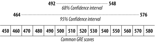
What does it mean to say that an observed score is most likely within one standard error of measurement of the true score? It is accepted by measurement statisticians that 68 percent of the time, an observed score will be within one standard error of measurement of the true score. Applied statisticians like to be more than 68 percent sure, however, and usually prefer to report a range of scores around the observed score that will contain the true score 95 percent of the time.
To be 95 percent sure that one is reporting a range of scores that contain an individual’s true score, one should report a range constructed by adding and subtracting about two standard errors of measurement. Figure 1-1 shows what confidence intervals around a score of 520 on the GRE Verbal test look like.
Why It Works
The procedure for building confidence intervals using the standard error of measurement is based on the assumptions that errors (or error scores) are random, and that these random errors are normally distributed. The normal curve [Hack #25] shows up here as it does all over the world of human characteristics, and its shape is well known and precisely defined. This precision allows for the calculation of precise confidence intervals.
The standard error of measurement is a standard deviation. In this case, it is the standard deviation of error scores around the true score. Under the normal curve, 68 percent of values are within one standard deviation of the mean, and 95 percent of scores are within about two standard deviations (more exactly, 1.96 standard deviations). It is this known set of probabilities that allows measurement folks to talk about 95 percent or 68 percent confidence.
What It Means
How is knowing the 95 percent confidence interval for a test score helpful? If you are the person who is requiring the test and using it to make a decision, you can judge whether the test taker is likely to be within reach of the level of performance you have set as your standard of success.
If you are the person who took the test, then you can be pretty sure that your true score is within a certain range. This might encourage you to take the test again with some reasonable expectation of how much better you are likely to do by chance alone. With your score of 520 on the GRE, you can be 95 percent sure that if you take the test again right away, your new score could be as high as 576. Of course, it could drop and be as low as 464 the next time, too.
Measure Up
Four levels of measurement determine how the scores produced in measurement can be used. If you have not measured at the right level, you might not be able to play with those scores the way you want.
Statistical procedures analyze numbers. The numbers must have meaning, of course; otherwise, the exercises are of little value. Statisticians call numbers with meaning scores. Not all the scores used in statistics, however, are created equal. Scores have different amounts of information in them, depending on the rules followed for creating the scores.
When you decide to measure something, you must choose the rules by which you assign scores very carefully. The level of measurement determines which sorts of statistical analyses are appropriate, which will work, and which will be meaningful.
Tip
Measurement is the meaningful assignment of numbers to things. The things can be concrete objects, such as rocks, or abstract concepts, such as intelligence.
Here’s an example of what I mean when I say not all scores are created equal. Imagine your five children took a spelling test. Chuck scored a 90, Dick and Jan got 80s, Bob scored 75, and Don got only 50 out of 100 correct. If a friend asked how your kids did on the big test, you might report that they averaged 75. This is a reasonable summary. Now, imagine that your five children ran a foot race against each other. Bob was first, Jan second, Dick third, Chuck fourth, and Don fifth. Your nosey friend again asks how they did. With a proud smile, you report that they averaged third place. This is not such a reasonable summary, because it provides no information. In both cases, though, scores were used to indicate performance. The difference lies only in the level of measurement used.
There are four levels of measurement—that is, four ways that numbers are used as scores. The levels differ in the amount of information provided and the types of mathematical and statistical analyses that can be meaningfully conducted on them. The four levels of measurement are nominal, ordinal,interval, and ratio.
Using Numbers as Labels
If you are planning to use scores to indicate only that the things belong to different groups, measure at the nominal level. The nominal level of measurement uses numbers only as names: labels for various categories (nominal means “in name only”).
For example, a scientist who collects data on men and women, using a 1 to indicate a male subject and a 2 to indicate a female subject, is using the numbers at a nominal level. Notice that even though the number 2 is mathematically greater than the number 1, a 2 in this data set does not mean more of anything. It is used only as a name.
Using Numbers to Show Sequence
If you want to analyze your scores in ways that rely on performance measured as evidence of some sequence or order, measure at the ordinal level. Ordinal measurement provides all the information the nominal level provides, but it adds information about the order of the scores. Numbers with greater values can be compared with numbers at lower values, and the people or otters or whatever was measured can be placed into a meaningful order.
Take, for example, your rank order in your high school class. The valedictorian is usually the person who received a score of 1 when grade point averages are compared. Notice that you can compare scores to each other, but you don’t know anything about the distance between the scores. In a footrace, the first-place finisher might have been just a second ahead of the second-place runner, while the second-place runner might have been 30 seconds ahead of the runner who came in third place.
Using Numbers to Show Distance
Interval level measurement uses numbers in a way that provides all the information of earlier levels, but adds an element of precision. This level of measurement produces scores that are interpreted as having an equal difference between any two adjacent scores.
For example, on a Fahrenheit thermometer, the meaningful difference between 70 and 69 degrees—1 degree—is equal to the difference between 32 and 31 degrees. That one degree is assumed to be the same amount of heat (or, if you prefer, pressure on the liquid in the thermometer), regardless of where on the scale the interval exists.
The interval level provides much more information than the ordinal level, and you can now meaningfully average scores. Most educational and psychological measurement takes place at the interval level.
Though interval level measurement would seem to solve all of our problems in terms of what we can and cannot do statistically, there are still some mathematical operations that are not meaningful at this level. For instance, we don’t make comparisons using fractions or proportions. Think about the way we talk about temperature. If a 40-degree day follows an 80-degree day, we do not say, “It is half as hot today as yesterday.” We also don’t refer to a student with a 120 IQ as “one-third smarter” than a student with a 90 IQ.
Tip
The word interval is a term from old-time castle architecture. You know those tall towers or turrets where archers were stationed for defense? Around the circular tops, there was typically a pattern of a protective stone, then a gap for launching arrows, followed by another protective stone, and so on. The gaps were called intervals (“between walls”), and the best designed defenses had the stones and gaps at equal intervals to provide 360-degree protection.
Using Numbers to Count in Concrete Ways
The highest level of measurement, ratio, provides all the information of the lower levels but also allows for proportional comparisons and the creation of percentages. Ratio level measurement is actually the most common and intuitive way in which we observe and take accounting of the natural world. When we count, we are at the ratio level. How many dogs are on your neighbor’s porch? The answer is at the ratio level.
Ratio level measurement provides so much information and allows for all possible statistical manipulations because ratio scales use a true zero. A true zero means that a person could score 0 on the scale and really have zero of the characteristic being measured. Though a Fahrenheit temperature scale, for example, does have a zero on it, a zero-degree day does not mean there is absolutely no heat. On interval scales, such as in our thermometer example, scores can be negative numbers. At the ratio level of measurement, there are no negative numbers.
Choosing Your Level of Measurement
Which level of measurement is right for you? Because of the advantages of moving to at least the interval level, most social scientists prefer to measure at the interval or ratio level. At the interval level, you can safely produce descriptive statistics and conduct inferential statistical analyses, such as t tests, analyses of variance, and correlational analyses. Table 1-6 provides a summary of the strengths and weaknesses of each level of measurement.
To choose the correct statistical analysis of data created by others, identify the level of measurement used and benefit from its strengths. If you are creating the data yourself, consider measuring up: using the highest level of measurement that you can.
Controversial Tools
Since the levels of measurement became commonly accepted in the 1950s, there has been some debate about whether we really need to clearly be at the interval level to conduct statistical analyses. There are many common forms of measurement (e.g., attitude scales, knowledge tests, or personality measures) that are not unequivocally at the interval level, but might be somewhere near the top of the ordinal level range. Can we safely use this level of data in analyses requiring interval scaling?
A majority consensus in the research literature is that if you are at least at the ordinal level and believe that you can make meaning out of interval-level statistical analyses, then you can safely perform inferential statistical analyses on this type of data. In the real world of research, by the way, almost everybody chooses this approach (whether they know it or not).
The basic value of making analytical decisions based on level of measurement is hard to deny, however. A classic example of the importance of measurement levels is described by Frederick Lord in his 1953 article “On the Statistical Treatment of Football Numbers” (American Psychologist, Vol. 8, 750-751). An absent-minded statistician eagerly analyzes some data given him concerning the college football team, and produces a report full of means and standard deviations and other sophisticated analyses. The data, though, turn out to be the numbers from the backs of the players’ jerseys. A clear instance of not paying attention to level of measurement, perhaps, but the statistician stands by his report. The numbers themselves, he explains, don’t know where they came from; they behave the same way regardless.
Power Up
Success in social science research is typically defined by the discovery of a statistically significant finding. To increase the chances of finding something, anything, the primary goal of the statistically savvy super-scientist should be to increase power.
There are two potential pitfalls when conducting statistically based research. Scientists might decide that they have found something in a population when it really exists only in their sample. Conversely, scientists might find nothing in their sample when, in reality, there was a beautiful relationship in the population just waiting to be found.
The first problem is minimized by sampling in a way that represents the population [Hack #19]. The second problem is solved by increasing power.
Power
In social science research, a statistical analysis frequently determines whether a certain value observed in a sample is likely to have occurred by chance. This process is called a test of significance. Tests of significance produce a p-value (probability value), which is the probability that the sample value could have been drawn from a particular population of interest.
The lower the p-value, the more confident we are in our beliefs that we have achieved statistical significance and that our data reveals a relationship that exists not only in our sample but also in the whole population represented by that sample. Usually, a predetermined level of significance is chosen as a standard for what counts. If the eventual p-value is equal to or lower than that predetermined level of significance, then the researcher has achieved a level of significance.
Tip
Statistical analyses and tests of significance are not limited to identifying relationships among variables, but the most common analyses (t tests, F tests, chi-squares, correlation coefficients, regression equations, etc.) usually serve this purpose. I talk about relationships here because they are the typical effect you’re looking for.
The power of a statistical test is the probability that, given that there is a relationship among variables in the population, the statistical analysis will result in the decision that a level of significance has been achieved. Notice this is a conditional probability. There must be a relationship in the population to find; otherwise, power has no meaning.
Power is not the chance of finding a significant result; it is the chance of finding that relationship if it is there to find. The formula for power contains three components:
Conducting a Power Analysis
Let’s say we want to compare two different sample groups and see whether they are different enough that there is likely a real difference in the populations they represent. For example, suppose you want to know whether men or women sleep more.
The design is fairly straightforward. Create two samples of people: one group of men and one group of women. Then, survey both groups and ask them the typical number of hours of sleep they get each night. To find any real differences, though, how many people do you need to survey? This is a power question.
Tip
A t test compares the mean performance of two sample groups of scores to see whether there is a significant difference [Hack #17]. In this case, statistical significance means that the difference between scores in the two populations represented by the two sample groups is probably greater than zero.
Before a study begins, a researcher can determine the power of the statistical analysis that will be used. Two of the three pieces needed to calculate power are already known before the study begins: you can decide the sample size and choose the predetermined level of significance. What you can’t know is the true size of the relationship between the variables, because data for the planned research has not yet been generated.
The size of the relationship among the variables of interest (i.e., the effect size) can be estimated by the researcher before the study begins; power also can be estimated before the study begins. Usually, the researcher decides on the smallest relationship size that would be considered important or interesting to find.
Once these three pieces (sample size, level of significance, and effect size) are determined, the fourth piece (power) can be calculated. In fact, setting the level of any three of these four pieces allows for calculation of the fourth piece. For example, a researcher often knows the power she would like an analysis to have, the effect size she wants to be declared statistically significant, and the preset level of significance she will choose. With this information, the researcher can calculate the necessary sample size.
Tip
For estimating power, researchers often use a standard accepted procedure that identifies a power goal of .80 and assigns a preset level of significance of .05. A power of .80 means that a researcher will find a relationship or effect in her sample 80 percent of the time if there is such a relationship in the population from which the sample was drawn.
The effect size (or index of relationship size [Hack #10]) with t tests is often expressed as the difference between the two means divided by the standard deviation in each group. This produces effect sizes in which .2 is considered small, .5 is considered medium, and .8 is considered large. The power analysis question is: how big a sample in each of the two groups (how many people) do I need in order to find a significant difference in test scores?
The actual formula for computing power is complex, and I won’t present it here. In real life, computer software or a series of dense tables in the back of statistics books are used to estimate power. I have done the calculations for a series of options, though, and present them in Table 1-7. Notice that the key variables are effect size and sample size. By convention, I have kept power at .80 and level of significance at .05.
| Effect size | Sample size |
| .10 | 1,600 |
| .20 | 400 |
| .30 | 175 |
| .40 | 100 |
| .50 | 65 |
| 1.0 | 20 |
Imagine that you think the actual difference in your gender-and-sleep study will be real, but small. A difference of about .2 standard deviations between groups in t test analyses is considered small, so you might expect a .2 effect size. To find that small of an effect size, you need 400 people in each group! As the effect size increases, the necessary sample size gets smaller. If the population effect size is 1.0 (a very large effect size and a big difference between the two groups), 20 people per group would suffice.
Making Inferences About Beautiful Relationships
Scientists often rely on the use of statistical inference to reject or accept their research hypotheses. They usually suggest a null hypothesis that says there is no relationship among variables or differences between groups. If their sample data suggests that there is, in fact, a relationship between their variables in the population, they will reject the null hypothesis [Hack #4] and accept the alternative, their research hypothesis, as the best guess about reality.
Of course, mistakes can be made in this process. Table 1-8 identifies the possible types of errors that can be made in this hypothesis-testing game. Rejecting the null hypothesis when you should not is called a Type I error by statistical philosophers. Failing to reject the null when you should is called a Type II error.
What you want to do as a smart scientist is avoid the two types of errors and produce a significant finding. Reaching a correct decision to not reject the null when the null is true is okay too, but not nearly as fun as a significant finding. “Spend your life in the upper-right quadrant of the table,” my Uncle Frank used to say, “and you will be happy and wealthy beyond your wildest dreams!”
To have a good chance of reaching a statistically significant finding, one condition beyond your control must be true. The null hypothesis must be false, or your chances of “finding” something are slim. And, if you do “find” something, it’s not really there, and you will be making a big error—a Type I error. There must actually be a relationship among your research variables in the population for you to find it in your sample data.
So, fate decides whether you wind up in the column on the right in Table 1-8. Power is the chance of moving to the top of that column once you get there. In other words, power is the chance of correctly rejecting the null hypothesis when the null hypothesis is false.
Why It Works
This relationship between effect size and sample size makes sense. Think of an animal hiding in a haystack. (The animal is the effect size; just work with me on this metaphor, please.) It takes fewer observations (handfuls of hay) to find a big ol’ effect size (like an elephant, say) than it would to find a tiny animal (like a cute baby otter, for instance). The number of people represents the number of observations, and big effect sizes hiding in populations are easier to find than smaller effect sizes.
The general relationship between effect size and sample size in power works the other way, too. Guess at your effect size, and just increase your sample size until you have the power you need. Remember, Table 1-7 assumes you want to have 80 percent power. You can always work with fewer people; you’ll just have less power.
Where It Doesn’t Work
It is important to remember that power is not the chance of success. It is not even the chance that a level of significance will be reached. It is the chance that a level of significance will be reached if all the values estimated by the researcher turn out to be correct. The hardest component of the formula to guess or set is the effect size in the population. A researcher seldom knows how big the thing is that he is looking for. After all, if he did know the size of the relationship between his research variables, there wouldn’t be much reason to conduct the study, would there?
Show Cause and Effect
Statistical researchers have established some ground rules that must be followed if you hope to demonstrate that one thing causes another.
Social science research that uses statistics operates under a couple of broad goals. One goal is to collect and analyze data about the world that will support or reject hypotheses about the relationships among variables. The second goal is to test hypotheses about whether there are cause-and-effect relationships among variables. The first goal is a breeze compared to the second.
There are all sorts of relationships between things in the world, and statisticians have developed all sorts of tools for finding them, but the presence of a relationship doesn’t mean that a particular variable causes another. Among humans, there is a pretty good positive correlation [Hack #11] between height and weight, for example, but if I lose a few pounds, I won’t get shorter. On the other hand, if I grow a few inches, I probably will gain some weight.
Knowing only the correlation between the two, however, can’t really tell me anything about whether one thing caused the other. Then again, the absence of a relationship would seem to tell me about cause and effect. If there is no correlation between two variables, that would seem to rule out the possibility that one causes the other. The presence of the correlation allows for that possibility, but does not prove it.
Designing Effective Experiments
Researchers have developed frameworks for talking about different research designs and whether such designs even allow for proof that one variable affects another. The different designs involve the presence or absence of comparison groups and how participants are assigned to those groups.
There are four basic categories of group designs, based on whether the design can provide strong evidence, moderate evidence, weak evidence, or no evidence of cause and effect:
- Non-experimental designs
These designs usually involve just one group of people, and statistics are used to either describe the population or demonstrate a relationship between variables. An example of this design is a correlational study, where simple associations among variables are analyzed [Hack #11]. This type of design provides no evidence of cause and effect.
- Pre-experimental designs
These designs usually involve one group of people and two or more measurement occasions to see whether change has occurred. An example of this design is to give a pretest to a group of people, do something to them, give them a post-test, and see whether their scores change. This type of design provides weak evidence of cause and effect because forces other than whatever you did to the poor folks could have caused any change in scores.
- Quasi-experimental designs
These designs involve more than one group of people, with at least one group acting as a comparison group. Assignment to these groups is not random but is determined by something outside the researcher’s control. An example of this design is comparing males and females on their attitudes toward statistics. At best, this sort of design provides moderate evidence of cause and effect. Without random assignment to groups, the groups are likely not equal on a bunch of unmeasured variables, and those might be the real cause for any differences that are found.
- Experimental designs
These designs have a comparison group and, importantly, people are assigned to the groups randomly. The random assignment to groups allows for researchers to assume that all groups are equal on all unmeasured variables, thus (theoretically) ruling them out as alternative explanations for any differences found. An example of this design is a drug study in which all participants randomly get either the drug being tested or a comparison drug or a placebo (sugar pill).
Does Weight Cause Height?
Earlier in this hack, I mentioned a well-known correlational finding: in people, height and weight tend to be related. Taller males weigh more, usually, then shorter males, for example. I laughed off the suggestion that if we fed people more, they would get taller—because of what I think I know about how the body grows, the suggestion that weight causes height is theoretically unlikely. But what if you demanded scientific proof?
I could test the hypothesis that weight causes height using a basic experimental design. Experimental designs have a comparison group, and the assignment to such groups must be random. Any relationships found under such circumstances are likely causal relationships. For my study, I’d create two groups:
- Group 1
Thirty college freshmen, who I would recruit from the population of the Midwestern university where I work. This group would be the experimental group; I would increase their weight and measure whether their height increases.
- Group 2
Thirty college freshmen, who I would recruit from the population of the Midwestern university where I work. This group would be the control group; I would not manipulate their weight at all and would then measure whether their height changes.
Tip
In this design, scientists would call weight the independent variable (because we don’t care what causes it) and height the dependent variable (because we wonder whether it depends on, or is caused by, the independent variable).
Because this design matches the criteria for experimental designs, we could interpret any relationships found as evidence of cause and effect.
Fighting Threats to Validity
Research conclusions fall into two types. They have to do with the cause-and-effect claim and whether any such claim, once it is established, is generalizable to whole populations or outside the laboratory. Table 1-9 displays the primary types of validity concerns when interpreting research results. These concerns are the hurdles that must be crossed by researchers.
| Validity concern | Validity question |
| Statistical conclusion validity | Is there a relationship among variables? |
| Internal validity | Is the relationship a cause-and-effect relationship? |
| Construct validity | Is the cause-and-effect relationship among the variables you believe should be affected? |
| External validity | Does this cause-and-effect relationship exist everywhere for everyone? |
Even when researchers have chosen a true experimental design, they still must worry that any results might not really be due to one variable affecting another. A cause-and-effect conclusion has many threats to its validity, but fortunately, just by thinking about it, researchers have identified many of these threats and have developed solutions.
Tip
Researchers’ understanding of group designs, the terminology used to describe them, the identification of threats to validity in research design, and the tools to guard against the threats are pretty much entirely due to the extremely influential works of Cook and Campbell, cited in the “See Also" section of this hack.
A few threats to the validity of causal claims and claims of generalizability are discussed next, along with some ways of eliminating them. There are dozens of threats identified and dealt with in the research design literature, but most of them are either unsolvable or can be solved with the same tools described here:
- History
Outside events could affect results. A solution is to use a control group (a comparison group that does not receive the drug or intervention or whatever), with random assignment of subjects to groups. Another part of the solution is to control both groups’ environments as much as possible (e.g., in laboratory-type settings).
- Maturation
Subjects develop naturally during a study, and changes might be due to these natural developments. Random assignment of participants to an experimental group and a control group solves this problem nicely.
- Selection
There might be systematic bias in assigning subjects to groups. The solution is to assign subjects randomly.
- Testing
Just taking a pretest might affect the level of the research variable. Create a comparison group and give both groups the pretest, so any changes will be equal between the groups. And assign subjects to the two groups randomly (are you starting to see a pattern here?).
- Instrumentation
There might be systematic bias in the measurement. The solution is to use valid, standardized, objectively scored tests.
- Hawthorne Effect
Subjects’ awareness that they are subjects in a study might affect results. To fight this, you could limit your subjects’ awareness of what results you expect, or you could conduct a double-blind study in which subjects (and researchers) don’t even know what treatment they are receiving.
The validity of research design and the validity of any claims about cause and effect are similar to claims of validity in measurement [Hack #28]. Such arguments are open and unending, and validity conclusions rest on a reasoned examination of the evidence at hand and consideration for what seems reasonable.
See Also
Campbell, D.T. and Stanley, J.C. (1966). Experimental and quasi-experimental designs for research. Chicago: Rand McNally.
Cook, T.D. and Campbell, D.T. (1979). Quasi-experimentation: Design and analysis issues for field settings. Boston: Houghton-Mifflin.
Shadish, W.R., Cook, T.D., and Campbell, D.T. (2002). Experimental and quasi-experimental designs for generalized causal inference. Boston: Houghton-Mifflin.
Know Big When You See It
You’ve just read about an amazing new scientific discovery, but is such a finding really a big deal? By applying effect size interpretations, you can judge the importance of such announcements (or lack thereof) for yourself.
Something is missing in most reports of scientific findings in nonscientific publications, on TV, on the radio, and—do I even have to mention—on the Web. Although reports in such media typically do a pretty good job of only reporting findings that are “statistically significant,” this is not enough to determine whether anything really important or useful has been discovered. A big drug study can report “significant” results, but still not have found anything of interest to the rest of us or even other researchers.
As we repeat in many places in this book, significance [Hack #4] means only that what you found is likely to be true about the bigger population you sampled from. The problem is that this fact alone is not nearly enough for you to know whether you should change your behavior, start a new diet, switch drugs, or reinterpret your view of the world.
What you need to know to make decisions about your life and reality in light of any new scientific report is the size of the relationship that has just been brought to light. How much better is brand A than brand B? How big is that SAT difference between boys and girls in meaningful terms? Is it worth it to take that half an aspirin a day, every day, to lower your risk of a heart attack? How much lower is that risk anyway?
The strength of that relationship should be expressed in some standardized way, too. Otherwise, there is no way to really judge how big it is. Using a statistical tool known as effect size will let you know big when you see it.
Seeing Effect Sizes Everywhere
An effect size is a standardized value that indicates the strength of a relationship between two variables. Before we talk about how to recognize or interpret effect sizes, let’s begin with some basics about relationships and statistical research.
Statistical research has always been interested in relationships among variables. The correlation coefficient, for example, is an index of the strength and direction of relationships between two sets of scores [Hack #11]. Less obvious, but still valid, examples of statistical procedures that measure relationships include t tests [Hack #17] and analysis of variance, a procedure for comparing more than two groups at one time.
Tip
Even procedures that compare different groups are still interested in relationships between variables. With a t test, for instance, a significant result means that it matters which group a person is in. In other words, there is an association between the independent variable (which defines the groups) and the dependent variable (the measured outcome).
Finding or Computing Effect Sizes
This hack is about finding and interpreting effect sizes to judge the implications of scientific findings reported in the popular media or in scientific writings. Often, the effect size is reported directly and you just have to know how to interpret it. Other times, it is not reported, but enough information is provided so that you can figure out what the effect size is.
When effect sizes are reported, they are typically one of three types. They differ depending on the procedure used and the way that procedure quantifies the information of interest. In each case, the effect size can be interpreted as estimates of the “size of the relationship between variables.” Here are the three typical types of effect sizes:
- Correlation coefficient
A correlation, symbolized by r, is already a measure of the relationship between variables and, thus, is an effect size. Because correlations can be negative, though, the value is sometimes squared to produce a value that is always greater than zero. Thus, the value of r 2 is interpreted as the “proportion of variance” shared by variables.
- d
This value, symbolized by d strangely enough, summarizes the difference between two group means used in a t test. It is calculated by dividing the mean difference of the two groups by the average standard deviation in the two groups.
Interpreting Effect Sizes
With levels of significance, statisticians have adopted certain sizes that are “good” to achieve. For example, most statistical researchers hope to achieve a .05 or lower level of significance. With effect sizes, though, there are not always certain values that are clearly good or clearly bad. Still, some standards for small, medium, and large effect sizes have been suggested.
The standards for big, medium, and little are based, for the most part, on the effect sizes that are normally found in real-world research. If a given effect size is so large as to be rarely found in published research, it is considered to be big. If the effect size is tiny and easy to find in real-life research, then it is considered to be small.
You should decide yourself, though, how big an effect size is of interest to you when interpreting research results. It all depends on the area of investigation. Table 1-10 provides the rules of thumb for how big is big.
Interpreting Research Findings
The advantage of talking about effect sizes when discussing research results is that everyone can get a sense of what impact the given research variable (or intervention, or drug, or teaching technique) is really having on the world. Because they are typically reported without any probability information (level of significance), effect sizes are most useful when provided alongside traditional level of significance numbers. This way, two questions can be answered:
Does this relationship probably exist in the population?
How big is the relationship?
Remember our example of whether you should decide to take half an aspirin each day to cut down your chances of having a heart attack? A well-publicized study in the late 1980s found a statistically significant relationship between these two variables. Of course, you should talk with your doctor before you make any sort of decision like this, but you should also have as much information as possible to help you make that decision. Let’s use effect size information to help us interpret these sorts of findings.
Here is what was reported in the media:
A sample of 22,071 physicians were randomly divided into two groups. For a long period of time, half took aspirin every day, while the other half took a placebo (which looked and tasted just like aspirin). At the end of the study period (which actually ended early because the effectiveness of aspirin was considered so large), the physicians taking aspirin were about half as likely to have had a heart attack than the placebo group. 1.71 percent of the placebo physicians had attacks versus about 1 percent (.94 percent) of the aspirin physicians. The findings were statistically significant.
The “clear” interpretation of such findings is that taking aspirin cuts your chances of a heart attack in half. Assuming that the study was representative and the physicians in the study are like you and me in important ways, this interpretation is fairly correct.
Another way to interpret the findings is to look at the effect size of the aspirin use. Using a formula for proportional comparisons, the effect size for this study is .06 standard deviations, or a d of .06. Applying the effect size standards shown in Table 1-10, this effect size should be interpreted as small—very small, really. This interpretation suggests that there is really quite a tiny relationship between aspirin-taking and heart attacks. The relationship is real, just not very strong.
One way to think about this is that your chances of having a heart attack during a given period of time is pretty small to begin with. 98.76 percent of everyone in the study did not have a heart attack, whether they took aspirin or not. Although taking aspirin does lower your chances, they go from small to a little smaller. It is similar to the idea that entering the lottery massively increases your chances of winning compared to those who do not enter, but your chances are still slim.
Why It Works
A researcher can achieve significant results, but still not have found anything for anyone to get excited about. This is because significance tells you only that your sample results probably did not occur by chance. The results are real and likely exist in the population. If you have found evidence of a small relationship between two variables or between the use of a drug and some medical outcome, the relationship might be so small that no one is really interested in it. The effect of the drug might be real, but weak, so it’s not worth recommending to patients. The relationship between A and B might be greater than zero, but so tiny as to do little to help understand either variable.
Modern researchers are still interested in whether there is statistical significance in their findings, but they should almost always report and discuss the effect size. If the effect size is reported, you can interpret it. If it is not reported, you can often dig out the information you need from published reports of scientific findings and calculate it yourself. The cool part is that you might then know more about the importance of the discovery than the media who reported the findings and, maybe, even the scientists themselves.
Get Statistics Hacks now with the O’Reilly learning platform.
O’Reilly members experience books, live events, courses curated by job role, and more from O’Reilly and nearly 200 top publishers.

