The purpose of this section is to serve as a kickoff point for subsequent discussions; it reviews some of the most basic aspects of the relational model as originally defined. Note that qualifier—“as originally defined”! One widespread misconception about the relational model is that it’s a totally static thing. It’s not. It’s like mathematics in that respect: Mathematics too is not a static thing but changes over time. In fact, the relational model can itself be seen as a small branch of mathematics; as such, it evolves over time as new theorems are proved and new results discovered. What’s more, those new contributions can be made by anyone who’s competent to do so; like other branches of mathematics, the relational model, though originally invented by one man, has become a community effort and now belongs to the world.
By the way, in case you don’t know, that one man was E. F. Codd, at the time a researcher at IBM (E for Edgar and F for Frank—but he always signed with his initials; to his friends, among whom I was proud to count myself, he was Ted). It was late in 1968 that Codd, a mathematician by training, first realized that the discipline of mathematics could be used to inject some solid principles and rigor into a field, database management, that prior to that time was all too deficient in any such qualities. His original definition of the relational model appeared in an IBM Research Report in 1969, and I’ll have a little more to say about that paper in Appendix G.
The original model had three major components—structure, integrity, and manipulation—and I’ll briefly describe each in turn. Please note right away, however, that all of the “definitions” I’ll be giving here are very loose; I’ll make them more precise as and when appropriate in later chapters.
First of all, then, structure. The principal structural feature is, of course, the relation itself, and as everybody knows it’s usual to picture relations on paper as tables (see Figure 1-1 below for a self-explanatory example). Relations are defined over types (also known as domains); a type is basically a conceptual pool of values from which actual attributes in actual relations take their actual values. With reference to the simple departments-and-employees database of Figure 1-1, for example, there might be a type called DNO (“department numbers”), which is the set of all valid department numbers, and then the attribute called DNO in the DEPT relation and the attribute called DNO in the EMP relation would both contain values from that conceptual pool. (By the way, it isn’t necessary—though it’s often a good idea—for attributes to have the same name as the corresponding type, and frequently they won’t. We’ll see plenty of counterexamples later.)
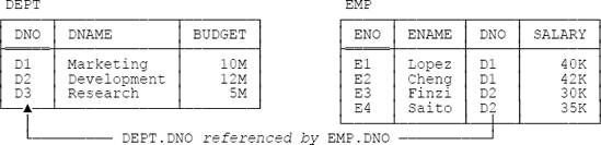
As I’ve said, tables like those in Figure 1-1 depict relations: n-ary relations, to be precise. An n-ary relation can be pictured as a table with n columns; the columns in that picture represent attributes of the relation and the rows represent tuples. The value n can be any nonnegative integer. A 1-ary relation is said to be unary; a 2-ary relation, binary; a 3-ary relation, ternary; and so on.
The relational model also supports various kinds of keys. To begin with—and this point is crucial!—every relation has at least one candidate key.[6] A candidate key is just a unique identifier; in other words, it’s a combination of attributes—often but not always a “combination” consisting of just a single attribute—such that every tuple in the relation has a unique value for the combination in question. In Figure 1-1, for example, every department has a unique department number and every employee has a unique employee number, so we can say that {DNO} is a candidate key for DEPT and {ENO} is a candidate key for EMP. Note the braces, by the way; to repeat, candidate keys are always combinations, or sets, of attributes (even when the set in question contains just one attribute), and the conventional representation of a set on paper is as a commalist of elements enclosed in braces.
Aside: This is the first time I’ve mentioned the useful term commalist, but I’ll be using it a lot in the pages ahead. It can be defined as follows: Let xyz be some syntactic construct (for example, “attribute name”). Then the term xyz commalist denotes a sequence of zero or more xyz’s in which each pair of adjacent xyz’s is separated by a comma (as well as, optionally, one or more spaces either before or after the comma or both). For example, if A, B, and C are attribute names, then the following are all attribute name commalists:
A , B , C
C , A , B
B
A , CSo too is the empty sequence of attribute names.
Moreover, when some commalist is enclosed in braces and thereby denotes a set, then (a) the order in which the elements appear within that commalist is immaterial (because sets have no ordering to their elements), and (b) if an element appears more than once, it’s treated as if it appeared just once (because sets don’t contain duplicate elements). End of aside.
Next, a primary key is a candidate key that’s been singled out for special treatment in some way. Now, if the relation in question has just one candidate key, then it doesn’t make any real difference if we decide to call that key “primary.” But if that relation has two or more candidate keys, then it’s usual to choose one of them as primary, meaning it’s somehow “more equal than the others.” Suppose, for example, that every employee always has both a unique employee number and a unique employee name—not a very realistic example, perhaps, but good enough for present purposes—so that {ENO} and {ENAME} are both candidate keys for EMP. Then we might choose {ENO}, say, to be the primary key.
Observe that I said it’s usual to choose a primary key. Indeed it is usual—but it’s not 100 percent necessary. If there’s just one candidate key, then there’s no choice and no problem; but if there are two or more, then having to choose one and make it primary smacks a little bit of arbitrariness (at least to me). Certainly there are situations where there don’t seem to be any good reasons for making such a choice. In this book, therefore, I usually will follow the primary key discipline—and in pictures like Figure 1-1 I’ll indicate primary key attributes by double underlining[7]—but I want to stress the fact that it’s really candidate keys, not primary keys, that are significant from a relational point of view. Partly for that reason, from this point forward I’ll use the term key, unqualified, to mean any candidate key, regardless of whether the candidate key in question has additionally been designated as “primary.” (In case you were wondering, the “special treatment” enjoyed by primary keys over other candidate keys is mainly syntactic in nature, anyway; it isn’t fundamental, and it isn’t very important.)
Finally, a foreign key is a combination, or set, of attributes FK in some relation r2 such that each FK value is required to be equal to some value of some key K in some relation r1 (r1and r2 not necessarily distinct).[8] With reference to Figure 1-1, for example, {DNO} is a foreign key in EMP whose values are required to match values of the key {DNO} in DEPT (as I’ve tried to suggest by means of a suitably labeled arrow in the figure). By required to match here, I mean that if, for example, EMP contains a tuple in which the DNO attribute has the value D2, then DEPT must also contain a tuple in which the DNO attribute has the value D2—for otherwise EMP would show some employee as being in a nonexistent department, and the database wouldn’t be “a faithful model of reality.”
An integrity constraint (constraint for short) is basically just a boolean expression that must evaluate to TRUE. In the case of departments and employees, for example, we might have a constraint to the effect that SALARY values must be greater than zero. Now, any given database will be subject to numerous constraints; however, all of those constraints will necessarily be specific to that database and will thus be expressed in terms of the relations in that database. By contrast, the relational model as originally formulated includes two generic constraints—generic, in the sense that they apply to every database, loosely speaking. One has to do with primary keys and the other with foreign keys. Here they are:
I’ll explain the second rule first. By the term unmatched foreign key value, I mean a foreign key value for which there doesn’t exist an equal value of the pertinent candidate key (the “target key”); thus, for example, the departments-and-employees database would be in violation of the referential integrity rule if it included an EMP tuple with a DNO value of D2, say, but no DEPT tuple with that same DNO value. So the referential integrity rule simply spells out the semantics of foreign keys; the name “referential integrity” derives from the fact that a foreign key value can be regarded as a reference to the tuple with that same value for the corresponding target key. In effect, therefore, the rule just says: If B references A, then A must exist.
As for the entity integrity rule, well, here I have a problem. The fact is, I reject the concept of “nulls” entirely; that is, it’s my very strong opinion that nulls have no place in the relational model. (Codd thought otherwise, obviously, but I have strong reasons for taking the position I do.) In order to explain the entity integrity rule, therefore, I need to suspend disbelief, as it were (at least for a few moments). Which I’ll now proceed to do ... but please understand that I’ll be revisiting the whole issue of nulls in Chapter 3 and Chapter 4.
In essence, then, a null is a “marker” that means value unknown. Crucially, it’s not itself a value; it is, to repeat, a marker, or flag. For example, suppose we don’t know employee E2’s salary. Then, instead of entering some real SALARY value in the tuple for employee E2 in relation EMP—we can’t enter a real value, by definition, precisely because we don’t know what that value should be—we mark the SALARY position within that tuple as null, as indicated here:
Now, it’s important to understand that this tuple contains nothing at all in the SALARY position. But it’s very hard to draw pictures of nothing at all! I’ve tried to show the SALARY position is empty in the picture above by shading it, but it would be more accurate not to show that position at all. Be that as it may, I’ll use this same convention of representing empty positions by shading elsewhere in this book—but that shading does not, to repeat, represent any kind of value at all. You can think of it (the shading, that is) as constituting the null “marker,” or flag, if you like.
To get back to the entity integrity rule: In terms of relation EMP, then, that rule says, loosely, that a given employee tuple might have an unknown name, or an unknown department number, or an unknown salary—but it can’t have an unknown employee number. The justification, such as it is, for this state of affairs is that if the employee number were unknown, we wouldn’t even know which “entity” (i.e., which employee) we were talking about.
That’s all I want to say about nulls for now. Please forget about them until further notice.
The manipulative part of the model in turn divides into two parts:
The relational assignment operator is fundamentally how updates are done in the relational model, and I’ll have more to say about it later, in the section RELATIONS vs. RELVARS. Note: I follow the usual convention throughout this book in using the generic term update to refer to the INSERT, DELETE, and UPDATE (and assignment) operators considered collectively. When I want to refer to the UPDATE operator specifically, I’ll set it in all caps as just shown.
As for the relational algebra, it consists of a set of operators that—speaking very loosely—allow us to derive “new” relations from “old” ones. Each such operator takes one or more relations as input and produces another relation as output; for example, difference (MINUS) takes two relations as input and “subtracts” one from the other, to derive another relation as output. And it’s very important that the output is another relation: That’s the well known closure property of the relational algebra. The closure property is what lets us write nested relational expressions; since the output from every operation is the same kind of thing as the input, the output from one operation can become the input to another. For example, we can take the difference r1 MINUS r2, feed the result as input to a union with some relation r3, feed that result as input to an intersection with some relation r4, and so on.
Now, any number of operators can be defined that fit the simple definition of “one or more relations in, exactly one relation out.” Here I’ll briefly describe what are usually thought of as the original operators (essentially the ones that Codd defined in his earliest papers);[9] I’ll give more details in Chapter 6, and in Chapter 7 I’ll describe a number of additional operators as well. Figure 1-2 is a pictorial representation of those original operators.
Note: If you’re unfamiliar with these operators and find the descriptions a little hard to follow, don’t worry about it; as I’ve already said, I’ll be going into much more detail, with lots of examples, in later chapters.

- Restrict
Returns a relation containing all tuples from a specified relation that satisfy a specified condition. For example, we might restrict relation EMP to just those tuples where the DNO value is D2.
- Project
Returns a relation containing all (sub)tuples that remain in a specified relation after specified attributes have been removed. For example, we might project relation EMP on just the ENO and SALARY attributes (thereby removing the ENAME and DNO attributes).
- Product
Returns a relation containing all possible tuples that are a combination of two tuples, one from each of two specified relations. Note: This operator is also known variously as cartesian product (sometimes extended or expanded cartesian product), cross product, cross join, and cartesian join; in fact, it’s really just a special case of join, as we’ll see in Chapter 6.
- Intersect
Returns a relation containing all tuples that appear in both of two specified relations. (Actually intersect, like product, is also a special case of join, as we’ll see in Chapter 6.)
- Union
Returns a relation containing all tuples that appear in either or both of two specified relations.
- Difference
Returns a relation containing all tuples that appear in the first and not the second of two specified relations.
- Join
Returns a relation containing all possible tuples that are a combination of two tuples, one from each of two specified relations, such that the two tuples contributing to any given result tuple have a common value for the common attributes of the two relations (and that common value appears just once, not twice, in that result tuple). Note: This kind of join was originally called the natural join, to distinguish it from various other kinds to be discussed later in this book. Since natural join is far and away the most important kind, however, it’s become standard practice to take the unqualified term join to mean the natural join specifically, and I’ll follow that practice in this book.
One last point to close this subsection: As you probably know, there’s also something called the relational calculus. The relational calculus can be regarded as an alternative to the relational algebra; that is, instead of saying the manipulative part of the relational model consists of the relational algebra (plus relational assignment), we can equally well say it consists of the relational calculus (plus relational assignment). The two are equivalent and interchangeable, in the sense that for every algebraic expression there’s a logically equivalent expression of the calculus and vice versa. I’ll have more to say about the calculus later, mostly in Chapter 10 and Chapter 11.
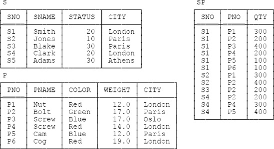
I’ll finish up this brief review by introducing the example I’ll be using as a basis for most if not all of the discussions in the rest of the book: the familiar—not to say hackneyed—suppliers-and-parts database. (I apologize for dragging out this old warhorse yet one more time, but I believe that using the same example in a variety of books and other publications can help, not hinder, learning.) Sample values are shown in Figure 1-3. To elaborate:
- Suppliers
Relation S denotes suppliers (more accurately, suppliers under contract). Each supplier has one supplier number (SNO), unique to that supplier (as you can see from the figure, I’ve made {SNO} the primary key); one name (SNAME), not necessarily unique (though the SNAME values in Figure 1-3 do happen to be unique); one status value (STATUS), representing some kind of ranking or preference level among available suppliers; and one location (CITY).
- Parts
Relation P denotes parts (more accurately, kinds of parts). Each kind of part has one part number (PNO), which is unique ({PNO} is the primary key); one name (PNAME); one color (COLOR); one weight (WEIGHT); and one location where parts of that kind are stored (CITY).
- Shipments
Relation SP denotes shipments (it shows which parts are supplied, or shipped, by which suppliers). Each shipment has one supplier number (SNO), one part number (PNO), and one quantity (QTY). For the sake of the example, I assume there’s at most one shipment at any given time for a given supplier and a given part ({SNO,PNO} is the primary key; also, {SNO} and {PNO} are both foreign keys, corresponding to the primary keys of S and P, respectively). Notice that the database of Figure 1-3 includes one supplier, supplier S5, with no shipments at all.
[6] Strictly speaking, this sentence should read “Every relvar has at least one candidate key” (see the section RELATIONS vs. RELVARS, later). Note: Actually, a similar remark applies elsewhere in this chapter as well. Exercise 1.1 at the end of the chapter addresses this issue.
Get SQL and Relational Theory, 2nd Edition now with the O’Reilly learning platform.
O’Reilly members experience books, live events, courses curated by job role, and more from O’Reilly and nearly 200 top publishers.

