As its name would imply, the role of an IGP is to provide routing connectivity within or interior to a given routing domain (RD). An RD is defined as a set of routers under common administrative control that share a common routing protocol. An enterprise network, which can also be considered an autonomous system (AS), may consist of multiple RDs, which may result from the (historic) need for multiple routed protocols, scaling limitations, acquisitions and mergers, or even a simple lack of coordination among organizations making up the enterprise. Route redistribution, the act of exchanging routing information among distinct routing protocols, is often performed to tie these RDs together when connectivity is desired.
IGP functions to advertise and learn network prefixes (routes) from neighboring routers to build a route table that ultimately contains entries for all sources advertising reachability for a given prefix. A route selection algorithm is executed to select the best (i.e., the shortest) path between the local router and each destination, and the next hop associated with that path is pushed into the forwarding table to affect the forwarding of packets that longest-match against that route prefix. The IGP wants to provide full connectivity among the routers making up an RD. Generally speaking, IGPs function to promote, not limit, connectivity, which is why we do not see IGPs used between ASsâthey lack the administrative controls needed to limit connectivity based on routing policy. This is also why inter-AS routing is normally accomplished using an Exterior Gateway Protocol (EGP), which today takes the form of Border Gateway Protocol (BGP) version 4. We discuss enterprise application of BGP in Chapter 5.
When network conditions change, perhaps due to equipment failure or management activity, the IGP both generates and receives updates and recalculates a new best route to the affected destinations. Here, the concept of a âbestâ route is normally tied to a route metric, which is the criterion used to determine the relative path of a given route. Generally speaking, a route metric is significant only to the routing protocol itâs associated with, and it is meaningful only within a given RD. In some cases, a router may learn multiple paths to an identical destination from more than one routing protocol. Given that metric comparison between two different IGPs is meaningless, the selection of the best route between multiple routing sources is controlled by a route preference. The concept of route preference is explored in detail later in this chapter in "IGP Migration: Common Techniques and Concerns" and is also known as administrative distance (AD) on Cisco Systems routers.
In addition to advertising internal network reachability, IGPs are
often used to advertise routing information that is external to that IGPâs
RD through a process known as route redistribution.
Route redistribution is often used to exchange routing information between
RDs to provide intra-AS connectivity. Route redistribution can be tricky
because mistakes can easily lead to lack of connectivity (black holes) or,
worse yet, routing loops. To ensure identical forwarding paths, you may
also need to map the metrics used by each routing protocol to ensure that
they are meaningful to the IGP into which they are redistributed. Route
redistribution is performed via routing policy in JUNOS software. We
introduce routing policy later in this chapter and cover it in detail in
Chapter 3. On Cisco Systems
platforms, redistribution is often performed through some combination of
the redistribute command, through
distribute lists, or through route maps and their associated IP access
lists. Although there is a learning curve, itâs often a delight for those
familiar with the IOS way of performing redistribution when they realize
that JUNOS software routing policy provides the same functionality with a
consistent set of semantics/syntax, for all protocols, and all in one
place!
The reader of this book is assumed to have an intermediate level understanding of the IP protocol and the general operation and characteristics of IGPs that support IP routing. This section provides a review of major characteristics, benefits, and drawbacks of the IGPs discussed in this chapter to prepare the reader for the configuration and migration examples that follow.
RIP is one of the oldest IP routing protocols still in production network use and is a true case of âif something works, why fix it?â The original specification for RIP (version 1) is defined in RFC 1058, originally published in June 1988! RIP version 2 (RIPv2) was originally defined in RFC 1388 (1993) and is currently specified in RFC 2453 (1998).
RIP is classified as a Distance Vector (DV) routing protocol because it advertises reachability information in the form of distance/vector pairsâwhich is to say that each route is represented as a cost (distance) to reach a given prefix (vector) tuple. DV routing protocols typically exchange entire route tables among their set of directly connected peers, on a periodic basis. This behavior, although direct and easy to understand, leads to many of the disadvantages associated with DV routing protocols. Specifically:
Increased network bandwidth consumption stemming from the periodic exchange of potentially large route tables, even during periods of network stability. This can be a significant issue when routers connect over low-speed or usage-based network services.
Slow network convergence, and as a result, a propensity to produce routing loops when reconverging around network failures. To alleviate (but not eliminate) the potential for routing loops, mechanisms such as split horizon, poisoned reverse, route hold downs, and triggered updates are generally implemented. These stability features come at the cost of prolonging convergence.
DV protocols are normally associated with crude route metrics that often will not yield optimal forwarding between destinations. The typical metric (cost) for DV protocols is a simple hop count, which is a crude measure of actual path cost, to say the least. For example, most users realize far better performance when crossing several routers interconnected by Gigabit Ethernet links, as opposed to half as many routers connected over low-speed serial interfaces.
On the upside, DV protocols are relatively simple to implement, understand, configure, and troubleshoot, and they have been around forever, allowing many network engineers a chance to become proficient in their deployment. The memory and processing requirements for DV protocols are generally less than those of a link state (LS) routing protocol (more on that later).
To help illustrate what is meant by slow to converge, consider that the protocolâs architects ultimately defined a hop count (the number of routers that need to be crossed to reach a destination) of 16 to be infinity! Given the original performance of initial implementations, the designers believed that networks over 16 hops in dimension would not be able to converge in a manner considered practical for use in production networks; and those were 1980s networks, for which demanding applications such as Voice over IP were but a distant gleam in an as yet grade-school-attending C-coderâs eye. Setting infinity to a rather low value was needed because in some conditions, RIP can converge only by cycling through a series of route exchanges between neighbors, with each such iteration increasing the routeâs cost by one, until the condition is cleared by the metric reaching infinity and both ends finally agree that the route is not reachable. With the default 30-second update frequency, this condition is aptly named a slow count to infinity.
Hold downs serve to increase stability, at the expense of rapid convergence, by preventing installation of a route with a reachable metric, after that same route was recently marked as unreachable (cost = 16) by the local router. This behavior helps to prevent loops by keeping the local router from installing route information for a route that was originally advertised by the local router, and which is now being readvertised by another neighbor. Itâs assumed that the slow count to infinity will complete before the hold down expires, after which the router will be able to install the route using the lowest advertised cost.
Split horizon prevents the advertisement of routing information back over the interface from which it was learned, and poisoned reverse alters this rule to allow readvertisement back out the learning interface, as long as the cost is explicitly set to infinity: a case of âI can reach this destination, NOT!â This helps to avoid loops by making it clear to any receiving routers that they should not use the advertising router as a next hop for the prefix in question. This behavior is designed to avoid the need for a slow count to infinity that might otherwise occur because the explicit indication that âI cannot reach destination Xâ is less likely to lead to misunderstandings when compared to the absence of information associated with split horizon. To prevent unnecessary bandwidth waste that stems from bothering to advertise a prefix that you cannot reach, most RIP implementations use split horizon, except when a route is marked as unreachable, at which point it is advertised with a poisoned metric for some number of update intervals (typically three).
Triggered updates allow a router to generate event-driven as well as ongoing periodic updates, serving to expedite the rate of convergence as changes propagate quickly. When combined with hold downs and split horizon, a RIP network can be said to receive bad news fast while good news travels slow.
Although the original RIP version still works and is currently supported on Juniper Networks routers, itâs assumed that readers of this book will consider deploying only RIP version 2. Although the basic operation and configuration are the same, several important benefits are associated with RIPv2 and there are no real drawbacks (considering that virtually all modern routers support both versions and that RIPv2 messages can be made backward-compatible with v1 routers, albeit while losing the benefits of RIPv2 for those V1 nodes).
RIPv2âs support of Variable Length Subnet Masking/classless interdomain routing (VLSM/CIDR), combined with its ability to authenticate routing exchanges, has resulted in a breath of new life for our old friend RIP (pun intended). Table 4-1 provides a summary comparison of the two RIP versions.
Table 4-1. Comparing characteristics and capabilities of RIP and RIPv2
Characteristic | RIP | RIPv2 |
|---|---|---|
Metric | Hop count (16 max) | Hop count (16 max) |
Updates/hold down/route timeout | 30/120/180 seconds | 30/120/180 seconds |
Max prefixes per message | 25 | 25 (24 when authentication is used) |
Authentication | None | Plain text or Message Digest 5 (MD5) |
Broadcast/multicast | Broadcast to all nodes using all 1s, RIP-capable or not | Multicast only to RIPv2-capable routers using 224.0.0.9 (broadcast mode is configurable) |
Support for VLSM/CIDR | No, only classful routing is supported (no netmask in updates) | Yes |
Route tagging | No | Yes (useful for tracking a routeâs source; i.e., internal versus external) |
The OSPF routing protocol currently enjoys widespread use in both enterprise and service provider networks. If OSPF can meet the needs of the worldâs largest network operators, itâs safe to say that it should be more than sufficient for even the largest enterprise network. OSPF version 2 is defined in RFC 2328, but numerous other RFCs define enhanced capabilities for OSPF, such as support of not-so-stubby areas (NSSAs) in RFC 3101, Multiprotocol Label Switching (MPLS) Traffic Engineering Extensions (MPLS TE) in RFC 3630, and in RFC 3623, which defines graceful restart extensions that minimize data plane disruption when a neighboring OSPF router restarts. OSPF supports virtually all the features any enterprise could desire, including VLSM, authentication, switched circuit support (suppressed hellos), and MPLS TE extensions, among many more.
OSPF is classified as an LS routing protocol. This is because, unlike a DV protocol that exchanges its entire route table among directly connected neighbors, OSPF exchanges only information about the local routerâs links, and these updates are flooded to all routers in the same area. Flooding ensures that all the routers in the area receive the new update at virtually the same time. The result of this flooding is a link-state database (LSDB) that is replicated among all routers that belong to a given area. Database consistency is critical for proper operation and the assurance of loop-free forwarding topologies. OSPF meets this requirement through reliable link-state advertisement (LSA) exchanges that incorporate acknowledgment and retransmission procedures. Each router performs a Shortest Path First (SPF) calculation based on the Dijkstra algorithm, using itself as the root of the tree to compute a shortest-path graph containing nodes representing each router in the area, along with its associated links. The metrically shortest path to each destination is then computed, and that route is placed into the route table for consideration to become an active route by the path selection algorithm.
OSPF advertises and updates prefix information using LSA messages, which are sent only upon detection of a change in network reachability. LSAs are also reflooded periodically to prevent their being aged out by other routers. Typically, this occurs somewhere between 30 and 45 minutes, given the default 3,600-second LSA lifetime. In addition, rather than sending an entire route table or database, these LSAs carry only the essential set of information needed to describe the routerâs new LS. Upon sensing a change in their local LSDBs, other routers rerun the SPF and act accordingly.
OSPF dynamically discovers and maintains neighbors through generation of periodic hello packets. An adjacency is formed when two neighbors decide to synchronize their LSDBs to become routing peers. A router may choose to form an adjacency with only a subset of the neighbors that it discovers to help improve efficiency, as described in the subsequent section, "Neighbors and adjacencies.â
It should be no wonder that OSPF has dramatically improved convergence characteristics when one considers its event-driven flooding of small updates to all routers in an area. This is especially true when contrasted to RIPâs period exchange of the entire route table among directly connected neighbors, who then convey that information to their neighbors at the next scheduled periodic update.
The downside to all this increased performance is that CPU and memory load are increased in routers as compared to the same router running a DV protocol. This is because an LS router has to house both the LSDB and the resulting route table, and the router must compute these routes by executing an SPF algorithm each time the LSDB changes. Considering that router processing capability and memory tend to increase, while actual costs tend to decrease for the same unit of processing power, these drawbacks are a more-than-acceptable trade-off for the benefit of ongoing reduced network loading and rapid convergence. Another drawback to LS routing protocols is their relative complexity when compared to DV protocols, which can make their operation difficult to understand, which in turn can make fault isolation more difficult.
OSPF was designed to support Type of Service (ToS)-based routing, but this capability has not been deployed commercially. This means that a single route table is maintained, and that for each destination, a single path metric is computed. This metric is said to be dimensionless in that it serves only to indicate the relative goodness or badness of a path, with smaller numbers considered to be better. Exactly what is better cannot be determined from the OSPF metric, LSDB, or resulting route table. Whether the OSPF metric is set to reflect link speed (default), hop count, delay, reliability, or some combination thereof is a matter of administrative policy.
Previously, it was noted that OSPF dynamically discovers neighbors using a periodic exchange of hello packets. It should also be noted that OSPF contains sanity checks that prevent neighbor discovery (and therefore, adjacency formation) when parameters such as the hello time, area type, maximum transmission unit (MTU), or subnet mask are mismatched. The designers of the protocol felt it was much easier to troubleshoot a missing adjacency than the potential result of trying to operate with mismatched parameters, and having dealt with more than a few misconfigured OSPF networks, the protocol architects were absolutely right.
To maximize efficiency, OSPF does not form an adjacency with every neighbor that is detected, because the maintenance of an adjacency requires compute cycles and because on multiaccess networks such as LANs, a full mesh of adjacencies is largely redundant. On multiaccess networks, an election algorithm is performed to first elect a designated router (DR), and then a backup designated router (BDR). The DR functions to represent the LAN itself and forms an adjacency with the BDR and all other compatible neighbors (DRother) on the LAN segment. The DRother routers form two adjacencies across the LANâone to the DR and one to the BDR. The neighbor state for DRother neighbors on a DRother router itself is expected to remain in the âtwo-wayâ state. This simply means that the various DRothers have detected each other as neighbors, but an adjacency has not been formed.
The DR is responsible for flooding LSAs that reflect the connectivity of the LAN. This means that loss of one neighbor on a 12-node LAN results in a single LSA that is flooded by the DR, as opposed to each remaining router flooding its own LSA. The reduced flooding results in reduced network bandwidth consumption and reduced OSPF processing overhead. If the DR fails, the BDR will take over and a new BDR is elected.
OSPF elects a DR and BDR based on a priority setting, with a lower value indicating a lesser chance at winning the election; a setting of 0 prevents the router from ever becoming the DR. In the event of a tie, the router with the highest router ID (RID) takes the prize. The OSPF DR Election algorithm is nondeterministic and nonrevertive, which means that adding a new router with a higher, more preferred priority does not result in the overthrow of the existing DR. In other words, router priority matters only during active DR/BDR election. This behavior minimizes the potential for network disruption/LSA flooding when new routers are added to the network. Thus, the only way to guarantee that a given router is the DR is to either disable DR capability in all other routers (set their priority to 0), or ensure that the desired router is powered on first and never reboots. Where possible, the most stable and powerful router should be made the DR/BDR, and a router should ideally be the DR for only one network segment.
OSPF describes various router roles that govern their operation and impact the types of areas in which they are permitted. To become proficient with OSPF operation and network design, you must have a clear understanding of the differences between OSPF area types and between the LSAs permitted within each area:
- Internal router
Any router that has all its interfaces contained within a single area is an internal router. If attached to the backbone area, the router is also known as a backbone router.
- Backbone router
Any router with an attachment to area 0 (the backbone area) is considered a backbone router. This router may also be an internal or area border router depending on whether it has links to other, nonbackbone areas.
- Area border router (ABR)
A router with links in two or more areas is an ABR. The ABR is responsible for connecting OSPF areas to the backbone by conveying network summary information between the backbone and nonbackbone areas.
- Antonymous system boundary router (ASBR)
A router that injects external routing information into an OSPF domain is an ASBR.
As previously noted, LS protocols flood LSAs to all routers in the same area in order to create a replicated LSDB from which a route table is derived through execution of an SPF algorithm. The interplay of these processes can lead to a downward-scaling spiral in large networks, especially when there are large numbers of unstable links.
As the number of routers and router links within an area grows, so too does the size of the resulting LSDB. In addition, more links means a greater likelihood of an interface or route flap, which leads to greater need for flooding of LSAs. The increased probability of LSDB churn leads to an increased frequency of the SPF calculations that must be performed each time the LSDB changes (barring any SPF hold downs for back-to-back LSA change events). These conditions combine to form the downward spiral of increased flooding, larger databases, more frequent SPF runs, and a larger processing burden per SPF run, due to the large size of the LSDB.
But donât fear: OSPF tackles this problem through the support of areas, which provides a hierarchy of LSDBs. As a result, LSA flooding is now constrained to each area, and no one router has to carry LS for the entire RD. Because each area is associated with its own LSDB, a multiarea OSPF network will, for the average router, result in a smaller LSDB. Each router must maintain an LSDB only for its attached areas, and no one router need attach to every area. This is a key point, because in theory it means OSPF has almost unlimited scaling potential, especially when compared to nonhierarchical protocols such as Ciscoâs EIGRP or RIP. In addition, with fewer routers and links, there is a reduced likelihood of having to flood updated LSAs, which in turn means a reduced number of SPF runs are neededâwhen an SPF run is needed, it is now executed against a smaller LSDB, which yields a win-win for all involved.
Routers that connect to multiple areas are called ABRs and maintain an LSDB for each area to which they attach. An ABR has a greater processing burden than an internal router, by virtue of maintaining multiple LSDBs, but the processing burden associated with two small LSDBs can still be considerably less than that associated with a single, large database, for reasons cited earlier. It is common to deploy your most powerful routers to serve the role of ABRs, because these machines will generally have to work harder than a purely internal router, given that they must maintain an LSDB per attached area, and have the greater chance of a resulting SPF calculation. However, the trade-off is being able to use smaller, less powerful routers within each area (internal routers), because of the reduced LSDB size that results from a hierarchical OSPF design.
Interestingly, OSPF is truly link-state only within a single area due to the scope of LSA flooding being confined to a single area. An ABR runs SPF for each attached areaâs LSDB and then summarizes its intraarea LS costs into other areas in DV-like fashion. This behavior is the reason OSPF requires a backbone area that is designated as area 0âgenerally speaking, each ABR generates and receives summaries only from the backbone, which exists to provide a loop-free environment over which these summaries can be exchanged. Put another way, the backbone serves to prevent loop formation that could result from the information that is hidden by ABRs when they summarize the contents of their nonbackbone area LSDBs into simple distance/vector pairs. A router receiving a summary advertisement uses SPF against that areaâs LSDB to compute the shortest path to the router that generated the summary advertisement, and then it simply adds the summary cost, as originally calculated by the advertising router, to obtain the total path cost.
Having said all this, it is not unheard of to see large, globally spanning OSPF networks consisting of hundreds of routers successfully deployed within a single OSPF area. There simply are no hard rules regarding the age-old question of âhow many routers can I put into a single area,â because too many variables exist. In addition to a simple router count, one must also consider factors such as link count, link stability, router processing power, the percentage of external versus internal LSAs, and the general robustness of the protocolâs implementation. The significance of the latter should not be underestimated. A poorly implemented OSPF instance running on the worldâs fastest hardware will likely not perform very well, unless, of course, you consider the number of core files dumped and/or reboots per unit of time, which is a significant IGP benchmark. Seriously, itâs bad enough when one network node keeps rolling over to play dead, but itâs worse when instability in a single node rapidly ripples out to affect the operation of other routers, even those with well-behaved code.
OSPF defines several different area types. To truly understand OSPF operation, you must have a clear understanding of the differences between OSPF area types, and between the LSAs permitted within each area:
- Backbone
To ensure loop-free connectivity, OSPF maintains a special area called the backbone area, which should always be designated as area 0. All other OSPF areas should connect themselves to the backbone for interarea connectivity; normally, interarea traffic transits the backbone.
- Stub
Stub areas do not carry AS external advertisements, with the goal being a reduction of LSDB size for internal routers within that stub area. Because routers in a stub area see only LSAs that advertise routing information from within the OSPF RD, a default route is normally injected to provide reachability to external destinations. Stub area routers use the metrically closest ABR when forwarding to AS external prefixes.
- Totally stubby area
A totally stubby area is a stub area that only receives the default route from the backbone. Routers in the totally stubby area do not see OSPF internal routes from other OSPF areas. Their LSDBs represent their own area and the injected default route, which is now used to reach both AS external and interarea destinations.
- NSSAs
As noted previously, an OSPF stub area does not carry external routes, which means you cannot redistribute routes into a stub area because redistributed routes are always treated as AS externals in OSPF. An NSSA bends this rule and allows a special form of external route within the NSSA. Although an NSSA can originate AS externals into OSPF, external routes from other areas are still not permitted within the NSSA. This is a case of having oneâs cake (small LSDB due to not being burdened by externals from other areas) while eating it too (being allowed to burden other routers with the external routes you choose to generate). The NSSAâs ABRs can translate the special form of external route used in an NSSA for flooding over the rest of the OSPF domain.
- Transit areas
Transit areas pass traffic from one adjacent area to the backbone or to another area if the backbone is more than two hops away from an area.
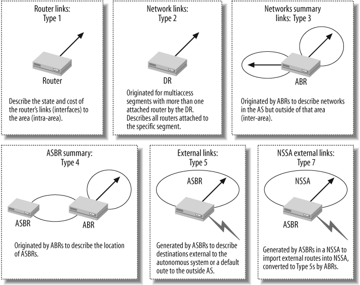
LSAs are the workhorse of OSPF in that they are used to flood information regarding network reachability and form the basis of the resulting LSDB. Table 4-2 describes the LSA types used by modern OSPF networks. It bears restating that a true understanding of OSPF requires knowledge of what type of routing information is carried in a given LSA, in addition to understanding each LSAâs flooding scope. For example, an LSA with area scope is never seen outside the area from which it was generated, whereas an LSA with global scope is flooded throughout the entire OSPF RD, barring any area type restrictions; that is, AS externals are never permitted within a stub area. Table 4-2 provides a graphical summary of the purpose and scope of the most common LSA types.
Table 4-2. Common OSPF LSA types
LSA type | Generated by/contents/purpose | Flooding scope |
|---|---|---|
Type 1, router | Generated by all OSPF routers, the Type 1 LSA describes the status and cost of the routerâs links. | Area |
Type 2, network | Generated by the DR on a LAN, the Type 2 LSA lists each router connected to the broadcast link, including the DR itself. | Area |
Type 3, network summary | Generated by ABRs, Type 3 LSAs carry summary route information between OSPF areas. Typically, this information is exchanged between a nonbackbone area and the backbone area, or vice versa. Type 3 LSAs are not reflooded across area boundaries; instead, a receiving ABR generates its own Type 3 LSA summarizing its interarea routing information into any adjacent areas. | Area |
Type 4, ASBR summary | Each ABR that forwards external route LSAs must also provide reachability information for the associated ASBR so that other routers know how to reach that ASBR when routing to the associated external destinations. The Type 4 LSA provides reachability information for the OSPF domainâs ASBRs. As with Type 3 LSAs, each ABR generates its own Type 4 when flooding external LSAs into another area. | Area |
Type 5, AS external LSA | Generated by ASBRs, the Type 5 LSA carries information for prefixes that are external to the OSPF RD. | Global, except for stub areas |
Type 7, NSSA | Generated by ASBRs in an NSSA, the Type 7 LSA advertises prefixes that are external to the OSPF RD. Unlike the Type 5 LSA, Type 7 LSAs are not globally flooded. Instead, the NSSAâs ABR translates Type 7 LSAs into Type 5 for flooding throughout the RD. | Area |
Type 9, 10, and 11, opaque LSAs | Generated by enabled OSPF routers to carry arbitrary information without having to define new LSA types, the Type 9 LSA has link scope and is currently used to support graceful restart extensions, whereas the Type 10 LSA has area scope and is used for MPLS TE support. | Type 9, link; Type 10, area; Type 11, global scope |
Breaking a large OSPF domain into multiple areas can have a significant impact on overall performance and convergence. In addition, most OSPF implementations support various timers to further tune and tweak the protocolâs operation.
The Juniper Networks OSPF implementation is quite optimized and lacks many of the timers and hold downs that readers may be familiar with in IOS. It is not uncommon to see users new to Juniper asking for JUNOS software analogs and receiving the standard answer that âthey do not exist because they are not needed.â The development engineers at Juniper feel that artificially delaying transmission of an LSAâostensibly to alleviate the processing burden associated with its receiptâdoes nothing except prolong network convergence.
Table 4-3 maps OSPF-related knobs from IOS to their JUNOS software equivalent, when available.
Table 4-3. IOS versus JUNOS software OSPF timers
IOS name | JUNOS software name | Comment |
|---|---|---|
|
| Delay notification of interface up/down events to damp interface transitions. Default is 0, but notification times can vary based on interrupt versus polled. |
|
| Control the rate of SPF calculation. In JUNOS software, the value is used for as many as three back-to-back SPF runs, and then a 5-second hold down is imposed to ensure stability in the network. |
| N/A | By default, JUNOS software sends 3 back-to-back updates with a 50 msec delay, and then a five-second hold down. |
| N/A | Controls the minimum interval for accepting a copy of the same LSA. |
|
| Delay back-to-back LSA transmissions out the same interface. |
| N/A | Enable incremental SPF calculations; JUNOS software does not support ISPF but does perform partial route calculations when the ospf topology is stable and only routing information changes. |
JUNOS software has added an additional optimization in the form of a periodic packet management process daemon (ppmd) that handles the generation and processing of OSPF (and other protocol) hello packets. The goal of ppmd is to permit scaling to large numbers of protocol peers by offloading the mundane processing tasks associated with periodic packet generation. The ppmd process can run directly in the PFE to offload RE cycles on application-specific integrated circuit (ASIC)-based systems such as the M7i.
In addition to the aforementioned timers, both vendors also support Bidirectional Forwarding Detection (BFD), which is a routing-protocol-agnostic mechanism to provide rapid detection of link failures, as opposed to waiting for an OSPF adjacency timeout. Note that interface hold time comes into play only when a physical layer fault is detected, as opposed to a link-level issue such as can occur when two routers are connected via a LAN switch, where the local interface status remains up even when a physical fault occurs on the remote link. As of this writing, IOS support for BFD is limited and varies by platform and software release; Cisco Systems recommends that you see the Cisco IOS software release notes for your software version to determine support and applicable restrictions.
The EIGRP is an updated version of Cisco Systemsâ proprietary IGRP. The original version of EIGRP had stability issues, prompting the release of EIGRP version 1, starting in IOS versions 10.3(11), 11.0(8), and 11.1(3). This chapter focuses strictly on EIGRP because it has largely displaced IGRP in modern enterprise networks.
EIGRP is sometimes said to be a âDV protocol that thinks itâs an LS.â EIGRP does in fact share some of the characteristics normally associated with LS routing, including rapid convergence and loop avoidance, but the lack of LSA flooding and the absence of the resulting LSDB expose EIGRPâs true DV nature. This section highlights the major operational characteristics and capabilities of EIGRP. The goal is not an exhaustive treatment of EIGRPâs operation or configurationâthis subject has been covered in numerous other writings. Instead, the purpose here is to understand EIGRP to the degree necessary to effectively replace this proprietary legacy protocol with another IGP, while maintaining maximum network availability throughout the process.
The operational characteristics of EIGRP are as follows:
It uses nonperiodic updates that are partial and bounded. This means that unlike typical DV protocol operation, EIGRP generates only triggered updates, that these updates report only affected prefixes, and that the updates are sent to a bounded set of neighbors.
It uses a Diffusing Update Algorithm (DUAL) to guarantee a loop-free topology while providing rapid convergence. The specifics of DUAL operation are outside the scope of this book; suffice it to say that DUAL is the muscle behind EIGRPâs rapid converge and loop guarantees.
It uses a composite metric that, by default, factors delay and throughput. Also, it supports the factoring of dynamically varying reliability and loading, but users are cautioned not to use this capability. EIGRP uses the same metric formula as IGRP, but it multiplies the result by 256 for greater granularity.
It supports VLSM/CIDR and automatic summarization at classful boundaries by default.
It supports unequal cost load balancing using a variance knob.
It supports neighbor discovery and maintenance using multicast.
It automatically redistributes to IGRP when process numbers are the same.
It features protocol-independent modules for common functionality (reliable transport of protocol messages).
It features protocol-dependant modules for IP, IPX, and AppleTalk that provide multiprotocol routing via the construction of separate route tables using protocol-specific routing updates.
At first glance, the multiprotocol capabilities of EIGRP may seem enticing. After all, this functionality cannot be matched by todayâs standardized routing protocols. There was a time when many enterprise backbones were in fact running multiple network protocols, and the lure of a single, high-performance IGP instance that could handle the three most common network suites was hard to resist. However, there has been an unmistakable trend toward IP transport for virtually all Internetworking suites, including IBMâs SNA/SAA. (We have a hard time recalling the last time we knew of an enterprise still deploying the native Netware or AppleTalk transport protocols.) In contrast, these proprietary-routed protocols are being phased out in favor of native IP transport, which serves to render EIGRPâs multiprotocol features moot in this modern age of IP internetworking.
EIGRP can load-balance across paths that are not equal in cost, based on a variance setting, which determines how much larger a path metric can be as compared to the minimum path metric, while still being used for load balancing. This characteristic remains unique to IGRP/EIGRP given that neither RIP nor OSPF supports unequal cost load balancing.
EIGRP uses a composite metric that lacks a direct corollary in standardized IGPs. EIGRP metrics tend to be large numbers. Although providing great granularity, these huge numbers represent a real issue for a protocol such as RIP, which sees any metric greater than 16 as infinity. Itâs quite unlikely that any enterprise would migrate from EIGRP to RIP anyway, given the relatively poor performance of RIP and the widespread availability of OSPF on modern networking devices, so such a transition scenario is not addressed in this chapter.
For reference, the formula used by EIGRP to calculate the metric is:
| Metric = [K1 * Bw + K2 * Bw/(256 - Load) + K3 * Delay] * [K5/(Reliability + K4)] |
Although the MTU is not used in the calculation of the metric, it is tracked across the path to identify the minimum path MTU. The K parameters are used to weigh each of the four components that factor into the composite metricânamely, bandwidth, load, delay, and reliability. The default values for the weighing result in only K1 and K3 being nonzero, which gives the default formula of Bw + Delay for the metric.
Tip
Note that Cisco Systems does not recommend user adjustment of the metric weighting. So, in practical terms, EIGRPâs metric is a 32-bit quantity that represents the pathâs cumulative delay (in tens of microseconds) and the pathâs minimum throughout in Kb/s, divided by 107 (scaled and inverted).
For EIGRP, the result is then multiplied by 256 to convert from IGRPâs 24-bit metric to EIGRPâs 32-bit metric. It should be obvious that one cannot perform a simple one-to-one mapping of legacy EIGRP metrics to OSPF, given that EIGRP supports a 32-bit metric and OSPFâs is only 16-bit. This is not a significant shortcoming in practice, given that few enterprise networks are composed of enough paths to warrant 4 billion levels of metric granularity anyway!
Figure 4-2 shows an example network to help illustrate how EIGRP calculates a path metric.
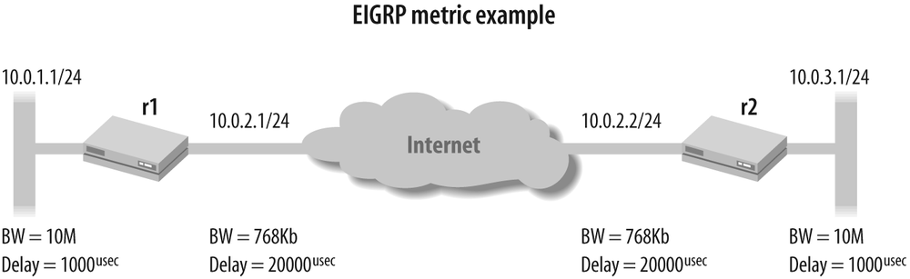
Using the default composite metric weighting for the topology
shown in Figure 4-2, router r1âs metric to reach 10.0.3.0/24 is computed
based on the minimum bandwidth and the sum of the path delay, using
the formula:
| Metric = 256 * (107/minBW Kbs) + (delay sum usec/10) |
Plugging in the specifics for this example yields a path metric
of 3,870,976 for the path to 10.0.3.0/24, from the perspective of
r1:
| Metric = 256 * (107/768) + (20,000 + 1,000 /10) |
| Metric = 256 * (13021) + (2100) |
| Metric = 256 * 15121 |
| Metric = 3,870,976 |
By way of comparison, the same network running OSPF with JUNOS software defaults for OSPF reference bandwidth yields a path metric of only 137! A key point here is that although 137 is certainly much smaller than the 3,870,976 value computed by EIGRP, the range of OSPF metrics, from 1â65,534, should be more than sufficient to differentiate among the number of links/paths available in even the largest enterprise network.
Also, recall that the OSPF metric is said to be dimensionless, which is to say that a smaller value is always preferred over larger values, but the exact nature of what is smaller is not conveyed in the metric itself. By default, OSPF derives its metric from interface bandwidth using a scaling factor, but the scaling factor can be altered, and the metric can be administratively assigned to reflect any parameter chosen by the administrator. When all is said and done, as long as a consistent approach is adopted when assigning OSPF metrics, the right thing should just happen. By way of example, consider a case where OSPF metrics are assigned based on the economic costs of a usage-based network service. The resultant shortest path measures distance as a function of economic impact and will result in optimization based on the least expensive paths between any two points. Thus, OSPF has done its job by locating the shortest path, which in this example means the least expensive path, given that the administration considers distance to equate to money. We revisit the subject of EIGRP to OSPF metric conversions in "EIGRP-to-OSPF Migration Summary,â later in this chapter.
Itâs worth restating that, unlike open standards protocols such as RIP and OSPF, EIGRP is proprietary to Cisco Systems. As a result, only Cisco Systems products can speak EIGRP, both because of the closed nature of the specification and because of the licensing and patent issues that prevent others from implementing the protocol. Most enterprise customers (and service providers, for that matter) prefer not to be locked into any solution that is sourced from a single vendor, even one as large and dominant as Cisco Systems.
EIGRPâs lack of hierarchical support significantly limits its use in large-scale networks due to scaling issues. EIGRP lacks the protocol extensions needed to build a traffic engineering database (TED), as used to support MPLS applications. Although MPLS is still somewhat rare in the enterprise, it currently enjoys significant momentum and is in widespread use within service provider networks across the globe. Considering that many of the requirements of service providers three or four years ago are the same requirements that we are seeing in the enterprise today, an enterprise would be wise to hedge its bets by adopting protocols that can support this important technology, should the need later arise.
Support is an important factor that must be considered when deploying any protocol. At one point, it was difficult to find off-the-shelf or open source protocol analysis for IGRP/EIGRP. Cisco could change the specification at any time, making obsolete any such tools that exist. At the time of this writing, the Wireshark analysis program (http://www.wireshark.org/) lists EIGRP support; however, itâs difficult to confirm the decode accuracy without an open standard to reference against.
Given the drawbacks to a single-vendor closed solution, an enterprise should consider the use of open standard protocols. In the case of IGPs, you gain higher performance, vendor independence, and off-the-shelf support capabilities. EIGRPâs multiprotocol capability aside, the largest IP networks on the planet (those of Internet service providers [ISPs]) generally run OSPF. Service provider networks are all about reliability, stability, rapid convergence at a large scale, and the ability to offer services that result in revenue generationâgiven these IGP requirements, the reader is left to ponder why service provider networks are never found to be running EIGRP within their networks.
IGPs provide the indispensable service of maintaining internal connectivity throughout the myriad link and equipment failures possible in modern IP internetworks. IGP performance and stability in the face of large volumes of network change can provide a strategic edge by quickly routing around problems to maintain the highest degree of connectivity possible.
This section overviewed the RIP, OSPF, and EIGRP protocols to prepare the reader for the following deployment and IGP migration scenarios. Now is a good time to take a break before you head into the RIP deployment case study that follows.
Get JUNOS Enterprise Routing now with the O’Reilly learning platform.
O’Reilly members experience books, live events, courses curated by job role, and more from O’Reilly and nearly 200 top publishers.

