Chapter 1. Meet Hadoop
In pioneer days they used oxen for heavy pulling, and when one ox couldn’t budge a log, they didn’t try to grow a larger ox. We shouldn’t be trying for bigger computers, but for more systems of computers.
—Grace Hopper
Data!
We live in the data age. It’s not easy to measure the total volume of data stored electronically, but an IDC estimate put the size of the “digital universe” at 0.18 zettabytes in 2006, and is forecasting a tenfold growth by 2011 to 1.8 zettabytes.[2] A zettabyte is 1021 bytes, or equivalently one thousand exabytes, one million petabytes, or one billion terabytes. That’s roughly the same order of magnitude as one disk drive for every person in the world.
This flood of data is coming from many sources. Consider the following:[3]
The New York Stock Exchange generates about one terabyte of new trade data per day.
Facebook hosts approximately 10 billion photos, taking up one petabyte of storage.
Ancestry.com, the genealogy site, stores around 2.5 petabytes of data.
The Internet Archive stores around 2 petabytes of data, and is growing at a rate of 20 terabytes per month.
The Large Hadron Collider near Geneva, Switzerland, will produce about 15 petabytes of data per year.
So there’s a lot of data out there. But you are probably wondering how it affects you. Most of the data is locked up in the largest web properties (like search engines), or scientific or financial institutions, isn’t it? Does the advent of “Big Data,” as it is being called, affect smaller organizations or individuals?
I argue that it does. Take photos, for example. My wife’s grandfather was an avid photographer, and took photographs throughout his adult life. His entire corpus of medium format, slide, and 35mm film, when scanned in at high-resolution, occupies around 10 gigabytes. Compare this to the digital photos that my family took last year, which take up about 5 gigabytes of space. My family is producing photographic data at 35 times the rate my wife’s grandfather’s did, and the rate is increasing every year as it becomes easier to take more and more photos.
More generally, the digital streams that individuals are producing are growing apace. Microsoft Research’s MyLifeBits project gives a glimpse of archiving of personal information that may become commonplace in the near future. MyLifeBits was an experiment where an individual’s interactions—phone calls, emails, documents—were captured electronically and stored for later access. The data gathered included a photo taken every minute, which resulted in an overall data volume of one gigabyte a month. When storage costs come down enough to make it feasible to store continuous audio and video, the data volume for a future MyLifeBits service will be many times that.
The trend is for every individual’s data footprint to grow, but perhaps more importantly the amount of data generated by machines will be even greater than that generated by people. Machine logs, RFID readers, sensor networks, vehicle GPS traces, retail transactions—all of these contribute to the growing mountain of data.
The volume of data being made publicly available increases every year too. Organizations no longer have to merely manage their own data: success in the future will be dictated to a large extent by their ability to extract value from other organizations’ data.
Initiatives such as Public Data Sets on Amazon Web Services, Infochimps.org, and theinfo.org exist to foster the “information commons,” where data can be freely (or in the case of AWS, for a modest price) shared for anyone to download and analyze. Mashups between different information sources make for unexpected and hitherto unimaginable applications.
Take, for example, the Astrometry.net project, which watches the Astrometry group on Flickr for new photos of the night sky. It analyzes each image, and identifies which part of the sky it is from, and any interesting celestial bodies, such as stars or galaxies. Although it’s still a new and experimental service, it shows the kind of things that are possible when data (in this case, tagged photographic images) is made available and used for something (image analysis) that was not anticipated by the creator.
It has been said that “More data usually beats better algorithms,” which is to say that for some problems (such as recommending movies or music based on past preferences), however fiendish your algorithms are, they can often be beaten simply by having more data (and a less sophisticated algorithm).[4]
The good news is that Big Data is here. The bad news is that we are struggling to store and analyze it.
Data Storage and Analysis
The problem is simple: while the storage capacities of hard drives have increased massively over the years, access speeds—the rate at which data can be read from drives—have not kept up. One typical drive from 1990 could store 1370 MB of data and had a transfer speed of 4.4 MB/s,[5] so you could read all the data from a full drive in around five minutes. Almost 20 years later one terabyte drives are the norm, but the transfer speed is around 100 MB/s, so it takes more than two and a half hours to read all the data off the disk.
This is a long time to read all data on a single drive—and writing is even slower. The obvious way to reduce the time is to read from multiple disks at once. Imagine if we had 100 drives, each holding one hundredth of the data. Working in parallel, we could read the data in under two minutes.
Only using one hundredth of a disk may seem wasteful. But we can store one hundred datasets, each of which is one terabyte, and provide shared access to them. We can imagine that the users of such a system would be happy to share access in return for shorter analysis times, and, statistically, that their analysis jobs would be likely to be spread over time, so they wouldn’t interfere with each other too much.
There’s more to being able to read and write data in parallel to or from multiple disks, though.
The first problem to solve is hardware failure: as soon as you start using many pieces of hardware, the chance that one will fail is fairly high. A common way of avoiding data loss is through replication: redundant copies of the data are kept by the system so that in the event of failure, there is another copy available. This is how RAID works, for instance, although Hadoop’s filesystem, the Hadoop Distributed Filesystem (HDFS), takes a slightly different approach, as you shall see later.
The second problem is that most analysis tasks need to be able to combine the data in some way; data read from one disk may need to be combined with the data from any of the other 99 disks. Various distributed systems allow data to be combined from multiple sources, but doing this correctly is notoriously challenging. MapReduce provides a programming model that abstracts the problem from disk reads and writes, transforming it into a computation over sets of keys and values. We will look at the details of this model in later chapters, but the important point for the present discussion is that there are two parts to the computation, the map and the reduce, and it’s the interface between the two where the “mixing” occurs. Like HDFS, MapReduce has reliability built-in.
This, in a nutshell, is what Hadoop provides: a reliable shared storage and analysis system. The storage is provided by HDFS, and analysis by MapReduce. There are other parts to Hadoop, but these capabilities are its kernel.
Comparison with Other Systems
The approach taken by MapReduce may seem like a brute-force approach. The premise is that the entire dataset—or at least a good portion of it—is processed for each query. But this is its power. MapReduce is a batch query processor, and the ability to run an ad hoc query against your whole dataset and get the results in a reasonable time is transformative. It changes the way you think about data, and unlocks data that was previously archived on tape or disk. It gives people the opportunity to innovate with data. Questions that took too long to get answered before can now be answered, which in turn leads to new questions and new insights.
For example, Mailtrust, Rackspace’s mail division, used Hadoop for processing email logs. One ad hoc query they wrote was to find the geographic distribution of their users. In their words:
This data was so useful that we’ve scheduled the MapReduce job to run monthly and we will be using this data to help us decide which Rackspace data centers to place new mail servers in as we grow.[6]
By bringing several hundred gigabytes of data together and having the tools to analyze it, the Rackspace engineers were able to gain an understanding of the data that they otherwise would never have had, and, furthermore, they were able to use what they had learned to improve the service for their customers. You can read more about how Rackspace uses Hadoop in Chapter 14.
RDBMS
Why can’t we use databases with lots of disks to do large-scale batch analysis? Why is MapReduce needed?
The answer to these questions comes from another trend in disk drives: seek time is improving more slowly than transfer rate. Seeking is the process of moving the disk’s head to a particular place on the disk to read or write data. It characterizes the latency of a disk operation, whereas the transfer rate corresponds to a disk’s bandwidth.
If the data access pattern is dominated by seeks, it will take longer to read or write large portions of the dataset than streaming through it, which operates at the transfer rate. On the other hand, for updating a small proportion of records in a database, a traditional B-Tree (the data structure used in relational databases, which is limited by the rate it can perform seeks) works well. For updating the majority of a database, a B-Tree is less efficient than MapReduce, which uses Sort/Merge to rebuild the database.
In many ways, MapReduce can be seen as a complement to an RDBMS. (The differences between the two systems are shown in Table 1-1.) MapReduce is a good fit for problems that need to analyze the whole dataset, in a batch fashion, particularly for ad hoc analysis. An RDBMS is good for point queries or updates, where the dataset has been indexed to deliver low-latency retrieval and update times of a relatively small amount of data. MapReduce suits applications where the data is written once, and read many times, whereas a relational database is good for datasets that are continually updated.
| Traditional RDBMS | MapReduce | |
| Data size | Gigabytes | Petabytes |
| Access | Interactive and batch | Batch |
| Updates | Read and write many times | Write once, read many times |
| Structure | Static schema | Dynamic schema |
| Integrity | High | Low |
| Scaling | Nonlinear | Linear |
Another difference between MapReduce and an RDBMS is the amount of structure in the datasets that they operate on. Structured data is data that is organized into entities that have a defined format, such as XML documents or database tables that conform to a particular predefined schema. This is the realm of the RDBMS. Semi-structured data, on the other hand, is looser, and though there may be a schema, it is often ignored, so it may be used only as a guide to the structure of the data: for example, a spreadsheet, in which the structure is the grid of cells, although the cells themselves may hold any form of data. Unstructured data does not have any particular internal structure: for example, plain text or image data. MapReduce works well on unstructured or semi-structured data, since it is designed to interpret the data at processing time. In other words, the input keys and values for MapReduce are not an intrinsic property of the data, but they are chosen by the person analyzing the data.
Relational data is often normalized to retain its integrity, and remove redundancy. Normalization poses problems for MapReduce, since it makes reading a record a nonlocal operation, and one of the central assumptions that MapReduce makes is that it is possible to perform (high-speed) streaming reads and writes.
A web server log is a good example of a set of records that is not normalized (for example, the client hostnames are specified in full each time, even though the same client may appear many times), and this is one reason that logfiles of all kinds are particularly well-suited to analysis with MapReduce.
MapReduce is a linearly scalable programming model. The programmer writes two functions—a map function and a reduce function—each of which defines a mapping from one set of key-value pairs to another. These functions are oblivious to the size of the data or the cluster that they are operating on, so they can be used unchanged for a small dataset and for a massive one. More importantly, if you double the size of the input data, a job will run twice as slow. But if you also double the size of the cluster, a job will run as fast as the original one. This is not generally true of SQL queries.
Over time, however, the differences between relational databases and MapReduce systems are likely to blur. Both as relational databases start incorporating some of the ideas from MapReduce (such as Aster Data’s and Greenplum’s databases), and, from the other direction, as higher-level query languages built on MapReduce (such as Pig and Hive) make MapReduce systems more approachable to traditional database programmers.[7]
Grid Computing
The High Performance Computing (HPC) and Grid Computing communities have been doing large-scale data processing for years, using such APIs as Message Passing Interface (MPI). Broadly, the approach in HPC is to distribute the work across a cluster of machines, which access a shared filesystem, hosted by a SAN. This works well for predominantly compute-intensive jobs, but becomes a problem when nodes need to access larger data volumes (hundreds of gigabytes, the point at which MapReduce really starts to shine), since the network bandwidth is the bottleneck, and compute nodes become idle.
MapReduce tries to colocate the data with the compute node, so data access is fast since it is local.[8] This feature, known as data locality, is at the heart of MapReduce and is the reason for its good performance. Recognizing that network bandwidth is the most precious resource in a data center environment (it is easy to saturate network links by copying data around), MapReduce implementations go to great lengths to preserve it by explicitly modelling network topology. Notice that this arrangement does not preclude high-CPU analyses in MapReduce.
MPI gives great control to the programmer, but requires that he or she explicitly handle the mechanics of the data flow, exposed via low-level C routines and constructs, such as sockets, as well as the higher-level algorithm for the analysis. MapReduce operates only at the higher level: the programmer thinks in terms of functions of key and value pairs, and the data flow is implicit.
Coordinating the processes in a large-scale distributed computation is a challenge. The hardest aspect is gracefully handling partial failure—when you don’t know if a remote process has failed or not—and still making progress with the overall computation. MapReduce spares the programmer from having to think about failure, since the implementation detects failed map or reduce tasks and reschedules replacements on machines that are healthy. MapReduce is able to do this since it is a shared-nothing architecture, meaning that tasks have no dependence on one other. (This is a slight oversimplification, since the output from mappers is fed to the reducers, but this is under the control of the MapReduce system; in this case, it needs to take more care rerunning a failed reducer than rerunning a failed map, since it has to make sure it can retrieve the necessary map outputs, and if not, regenerate them by running the relevant maps again.) So from the programmer’s point of view, the order in which the tasks run doesn’t matter. By contrast, MPI programs have to explicitly manage their own checkpointing and recovery, which gives more control to the programmer, but makes them more difficult to write.
MapReduce might sound like quite a restrictive programming model, and in a sense it is: you are limited to key and value types that are related in specified ways, and mappers and reducers run with very limited coordination between one another (the mappers pass keys and values to reducers). A natural question to ask is: can you do anything useful or nontrivial with it?
The answer is yes. MapReduce was invented by engineers at Google as a system for building production search indexes because they found themselves solving the same problem over and over again (and MapReduce was inspired by older ideas from the functional programming, distributed computing, and database communities), but it has since been used for many other applications in many other industries. It is pleasantly surprising to see the range of algorithms that can be expressed in MapReduce, from image analysis, to graph-based problems, to machine learning algorithms.[9] It can’t solve every problem, of course, but it is a general data-processing tool.
You can see a sample of some of the applications that Hadoop has been used for in Chapter 14.
Volunteer Computing
When people first hear about Hadoop and MapReduce, they often ask, “How is it different from SETI@home?” SETI, the Search for Extra-Terrestrial Intelligence, runs a project called SETI@home in which volunteers donate CPU time from their otherwise idle computers to analyze radio telescope data for signs of intelligent life outside earth. SETI@home is the most well-known of many volunteer computing projects; others include the Great Internet Mersenne Prime Search (to search for large prime numbers) and Folding@home (to understand protein folding, and how it relates to disease).
Volunteer computing projects work by breaking the problem they are trying to solve into chunks called work units, which are sent to computers around the world to be analyzed. For example, a SETI@home work unit is about 0.35 MB of radio telescope data, and takes hours or days to analyze on a typical home computer. When the analysis is completed, the results are sent back to the server, and the client gets another work unit. As a precaution to combat cheating, each work unit is sent to three different machines, and needs at least two results to agree to be accepted.
Although SETI@home may be superficially similar to MapReduce (breaking a problem into independent pieces to be worked on in parallel), there are some significant differences. The SETI@home problem is very CPU-intensive, which makes it suitable for running on hundreds of thousands of computers across the world,[10] since the time to transfer the work unit is dwarfed by the time to run the computation on it. Volunteers are donating CPU cycles, not bandwidth.
MapReduce is designed to run jobs that last minutes or hours on trusted, dedicated hardware running in a single data center with very high aggregate bandwidth interconnects. By contrast, SETI@home runs a perpetual computation on untrusted machines on the Internet with highly variable connection speeds and no data locality.
A Brief History of Hadoop
Hadoop was created by Doug Cutting, the creator of Apache Lucene, the widely used text search library. Hadoop has its origins in Apache Nutch, an open source web search engine, itself a part of the Lucene project.
Building a web search engine from scratch was an ambitious goal, for not only is the software required to crawl and index websites complex to write, but it is also a challenge to run without a dedicated operations team, since there are so many moving parts. It’s expensive too: Mike Cafarella and Doug Cutting estimated a system supporting a 1-billion-page index would cost around half a million dollars in hardware, with a monthly running cost of $30,000.[12] Nevertheless, they believed it was a worthy goal, as it would open up and ultimately democratize search engine algorithms.
Nutch was started in 2002, and a working crawler and search system quickly emerged. However, they realized that their architecture wouldn’t scale to the billions of pages on the Web. Help was at hand with the publication of a paper in 2003 that described the architecture of Google’s distributed filesystem, called GFS, which was being used in production at Google.[13] GFS, or something like it, would solve their storage needs for the very large files generated as a part of the web crawl and indexing process. In particular, GFS would free up time being spent on administrative tasks such as managing storage nodes. In 2004, they set about writing an open source implementation, the Nutch Distributed Filesystem (NDFS).
In 2004, Google published the paper that introduced MapReduce to the world.[14] Early in 2005, the Nutch developers had a working MapReduce implementation in Nutch, and by the middle of that year all the major Nutch algorithms had been ported to run using MapReduce and NDFS.
NDFS and the MapReduce implementation in Nutch were applicable beyond the realm of search, and in February 2006 they moved out of Nutch to form an independent subproject of Lucene called Hadoop. At around the same time, Doug Cutting joined Yahoo!, which provided a dedicated team and the resources to turn Hadoop into a system that ran at web scale (see sidebar). This was demonstrated in February 2008 when Yahoo! announced that its production search index was being generated by a 10,000-core Hadoop cluster.[15]
In January 2008, Hadoop was made its own top-level project at Apache, confirming its success and its diverse, active community. By this timem Hadoop was being used by many other companies besides Yahoo!, such as Last.fm, Facebook, and the New York Times (some applications are covered in the case studies in Chapter 14 and on the Hadoop wiki.
In one well-publicized feat, the New York Times used Amazon’s EC2 compute cloud to crunch through four terabytes of scanned archives from the paper converting them to PDFs for the Web.[16] The processing took less than 24 hours to run using 100 machines, and the project probably wouldn’t have been embarked on without the combination of Amazon’s pay-by-the-hour model (which allowed the NYT to access a large number of machines for a short period), and Hadoop’s easy-to-use parallel programming model.
In April 2008, Hadoop broke a world record to become the fastest system to sort a terabyte of data. Running on a 910-node cluster, Hadoop sorted one terabyte in 209 seconds (just under 3½ minutes), beating the previous year’s winner of 297 seconds (described in detail in TeraByte Sort on Apache Hadoop). In November of the same year, Google reported that its MapReduce implementation sorted one terabyte in 68 seconds.[17] As this book was going to press (May 2009), it was announced that a team at Yahoo! used Hadoop to sort one terabyte in 62 seconds.
The Apache Hadoop Project
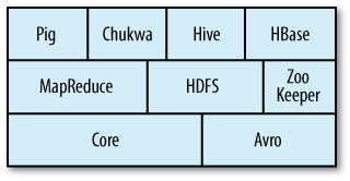
Today, Hadoop is a collection of related subprojects that fall under the umbrella of infrastructure for distributed computing. These projects are hosted by the Apache Software Foundation, which provides support for a community of open source software projects. Although Hadoop is best known for MapReduce and its distributed filesystem (HDFS, renamed from NDFS), the other subprojects provide complementary services, or build on the core to add higher-level abstractions. The subprojects, and where they sit in the technology stack, are shown in Figure 1-1 and described briefly here:
- Core
A set of components and interfaces for distributed filesystems and general I/O (serialization, Java RPC, persistent data structures).
- Avro
A data serialization system for efficient, cross-language RPC, and persistent data storage. (At the time of this writing, Avro had been created only as a new subproject, and no other Hadoop subprojects were using it yet.)
- MapReduce
A distributed data processing model and execution environment that runs on large clusters of commodity machines.
- HDFS
A distributed filesystem that runs on large clusters of commodity machines.
- Pig
A data flow language and execution environment for exploring very large datasets. Pig runs on HDFS and MapReduce clusters.
- HBase
A distributed, column-oriented database. HBase uses HDFS for its underlying storage, and supports both batch-style computations using MapReduce and point queries (random reads).
- ZooKeeper
A distributed, highly available coordination service. ZooKeeper provides primitives such as distributed locks that can be used for building distributed applications.
- Hive
A distributed data warehouse. Hive manages data stored in HDFS and provides a query language based on SQL (and which is translated by the runtime engine to MapReduce jobs) for querying the data.
- Chukwa
A distributed data collection and analysis system. Chukwa runs collectors that store data in HDFS, and it uses MapReduce to produce reports. (At the time of this writing, Chukwa had only recently graduated from a “contrib” module in Core to its own subproject.)
[2] From Gantz et al., “The Diverse and Exploding Digital Universe,” March 2008 (http://www.emc.com/collateral/analyst-reports/diverse-exploding-digital-universe.pdf).
[3] http://www.intelligententerprise.com/showArticle.jhtml?articleID=207800705, http://mashable.com/2008/10/15/facebook-10-billion-photos/, http://blog.familytreemagazine.com/insider/Inside+Ancestrycoms+TopSecret+Data+Center.aspx, and http://www.archive.org/about/faqs.php, http://www.interactions.org/cms/?pid=1027032.
[4] The quote is from Anand Rajaraman writing about the Netflix Challenge (http://anand.typepad.com/datawocky/2008/03/more-data-usual.html).
[5] These specifications are for the Seagate ST-41600n.
[7] In January 2007, David J. DeWitt and Michael Stonebraker caused a stir by publishing “MapReduce: A major step backwards” (http://www.databasecolumn.com/2008/01/mapreduce-a-major-step-back.html), in which they criticized MapReduce for being a poor substitute for relational databases. Many commentators argued that it was a false comparison (see, for example, Mark C. Chu-Carroll’s “Databases are hammers; MapReduce is a screwdriver,” http://scienceblogs.com/goodmath/2008/01/databases_are_hammers_mapreduc.php), and DeWitt and Stonebraker followed up with “MapReduce II” (http://www.databasecolumn.com/2008/01/mapreduce-continued.html), where they addressed the main topics brought up by others.
[8] Jim Gray was an early advocate of putting the computation near the data. See “Distributed Computing Economics,” March 2003, http://research.microsoft.com/apps/pubs/default.aspx?id=70001.
[9] Apache Mahout (http://lucene.apache.org/mahout/) is a project to build machine learning libraries (such as classification and clustering algorithms) that run on Hadoop.
[10] In January 2008, SETI@home was reported at http://www.planetary.org/programs/projects/setiathome/setiathome_20080115.html to be processing 300 gigabytes a day, using 320,000 computers (most of which are not dedicated to SETI@home; they are used for other things, too).
[11] In this book, we use the lowercase form, “jobtracker,” to
denote the entity when it’s being referred to generally, and the
CamelCase form JobTracker to denote the
Java class that implements it.
[12] Mike Cafarella and Doug Cutting, “Building Nutch: Open Source Search,” ACM Queue, April 2004, http://queue.acm.org/detail.cfm?id=988408.
[13] Sanjay Ghemawat, Howard Gobioff, and Shun-Tak Leung, “The Google File System,” October 2003, http://labs.google.com/papers/gfs.html.
[14] Jeffrey Dean and Sanjay Ghemawat, “MapReduce: Simplified Data Processing on Large Clusters ,” December 2004, http://labs.google.com/papers/mapreduce.html.
[15] “Yahoo! Launches World’s Largest Hadoop Production Application,” 19 February 2008, http://developer.yahoo.net/blogs/hadoop/2008/02/yahoo-worlds-largest-production-hadoop.html.
[16] Derek Gottfrid, “Self-service, Prorated Super Computing Fun!,” 1 November 2007, http://open.blogs.nytimes.com/2007/11/01/self-service-prorated-super-computing-fun/.
[17] “Sorting 1PB with MapReduce,” 21 November 2008, http://googleblog.blogspot.com/2008/11/sorting-1pb-with-mapreduce.html.
Get Hadoop: The Definitive Guide now with the O’Reilly learning platform.
O’Reilly members experience books, live events, courses curated by job role, and more from O’Reilly and nearly 200 top publishers.

