Chapter 4. Spam Filters, Naive Bayes, and Wrangling
The contributor for this chapter is Jake Hofman. Jake is at Microsoft Research after recently leaving Yahoo! Research. He got a PhD in physics at Columbia and regularly teaches a fantastic course on data-driven modeling at Columbia, as well as a newer course in computational social science.
As with our other presenters, we first took a look at Jake’s data science profile. It turns out he is an expert on a category that he added to the data science profile called “data wrangling.” He confessed that he doesn’t know if he spends so much time on it because he’s good at it or because he’s bad at it. (He’s good at it.)
Thought Experiment: Learning by Example
Let’s start by looking at a bunch of text shown in Figure 4-1, whose rows seem to contain the subject and first line of an email in an inbox.
You may notice that several of the rows of text look like spam.
How did you figure this out? Can you write code to automate the spam filter that your brain represents?
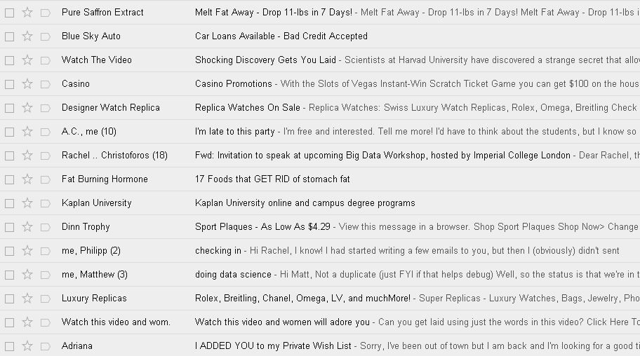
Figure 4-1. Suspiciously spammy
Rachel’s class had a few ideas about what things might be clear signs of spam:
-
Any email is spam if it contains Viagra references. That’s a good rule to start with, but as you’ve likely seen in your own email, people figured out this spam filter rule and got around it by modifying the spelling. (It’s sad that spammers are so smart and aren’t working on more important projects than selling lots of Viagra…)
-
Maybe something about the length of the subject gives it away as spam, or perhaps excessive use of exclamation points or other punctuation. But some words like “Yahoo!” are authentic, so you don’t want to make your rule too simplistic.
And here are a few suggestions regarding code you could write to identify spam:
-
Try a probabilistic model. In other words, should you not have simple rules, but have many rules of thumb that aggregate together to provide the probability of a given email being spam? This is a great idea.
-
What about k-nearest neighbors or linear regression? You learned about these techniques in the previous chapter, but do they apply to this kind of problem? (Hint: the answer is “No.”)
In this chapter, we’ll use Naive Bayes to solve this problem, which is in some sense in between the two. But first…
Why Won’t Linear Regression Work for Filtering Spam?
Because we’re already familiar with linear regression and that’s a tool in our toolbelt, let’s start by talking through what we’d need to do in order to try to use linear regression. We already know that’s not what we’re going to use, but let’s talk it through to get to why. Imagine a dataset or matrix where each row represents a different email message (it could be keyed by email_id). Now let’s make each word in the email a feature—this means that we create a column called “Viagra,” for example, and then for any message that has the word Viagra in it at least once, we put a 1 in; otherwise we assign a 0. Alternatively, we could put the number of times the word appears. Then each column represents the appearance of a different word.
Thinking back to the previous chapter, in order to use linear regression, we need to have a training set of emails where the messages have already been labeled with some outcome variable. In this case, the outcomes are either spam or not. We could do this by having human evaluators label messages “spam,” which is a reasonable, albeit time-intensive, solution. Another way to do it would be to take an existing spam filter such as Gmail’s spam filter and use those labels. (Now of course if you already had a Gmail spam filter, it’s hard to understand why you might also want to build another spam filter in the first place, but let’s just say you do.) Once you build a model, email messages would come in without a label, and you’d use your model to predict the labels.
The first thing to consider is that your target is binary (0 if not spam, 1 if spam)—you wouldn’t get a 0 or a 1 using linear regression; you’d get a number. Strictly speaking, this option really isn’t ideal; linear regression is aimed at modeling a continuous output and this is binary.
This issue is basically a nonstarter. We should use a model appropriate for the data. But if we wanted to fit it in R, in theory it could still work. R doesn’t check for us whether the model is appropriate or not. We could go for it, fit a linear model, and then use that to predict and then choose a critical value so that above that predicted value we call it “1” and below we call it “0.”
But if we went ahead and tried, it still wouldn’t work because there are too many variables compared to observations! We have on the order of 10,000 emails with on the order of 100,000 words. This won’t work. Technically, this corresponds to the fact that the matrix in the equation for linear regression is not invertible—in fact, it’s not even close. Moreover, maybe we can’t even store it because it’s so huge.
Maybe we could limit it to the top 10,000 words? Then we could at least have an invertible matrix. Even so, that’s too many variables versus observations to feel good about it. With carefully chosen feature selection and domain expertise, we could limit it to 100 words and that could be enough! But again, we’d still have the issue that linear regression is not the appropriate model for a binary outcome.
Aside: State of the Art for Spam Filters
In the last five years, people have started using stochastic gradient methods to avoid the noninvertible (overfitting) matrix problem. Switching to logistic regression with stochastic gradient methods helped a lot, and can account for correlations between words. Even so, Naive Bayes is pretty impressively good considering how simple it is.
How About k-nearest Neighbors?
We’re going to get to Naive Bayes shortly, we promise, but let’s take a minute to think about trying to use k-nearest neighbors (k-NN) to create a spam filter. We would still need to choose features, probably corresponding to words, and we’d likely define the value of those features to be 0 or 1, depending on whether the word is present or not. Then, we’d need to define when two emails are “near” each other based on which words they both contain.
Again, with 10,000 emails and 100,000 words, we’ll encounter a problem, different from the noninvertible matrix problem. Namely, the space we’d be working in has too many dimensions. Yes, computing distances in a 100,000-dimensional space requires lots of computational work. But that’s not the real problem.
The real problem is even more basic: even our nearest neighbors are really far away. This is called “the curse of dimensionality,” and it makes k-NN a poor algorithm in this case.
Naive Bayes
So are we at a loss now that two methods we’re familiar with, linear regression and k-NN, won’t work for the spam filter problem? No! Naive Bayes is another classification method at our disposal that scales well and has nice intuitive appeal.
Bayes Law
Let’s start with an even simpler example than the spam filter to get a feel for how Naive Bayes works. Let’s say we’re testing for a rare disease, where 1% of the population is infected. We have a highly sensitive and specific test, which is not quite perfect:
-
99% of sick patients test positive.
-
99% of healthy patients test negative.
Given that a patient tests positive, what is the probability that the patient is actually sick?
A naive approach to answering this question is this: Imagine we have 100 × 100 = 10,000 perfectly representative people. That would mean that 100 are sick, and 9,900 are healthy. Moreover, after giving all of them the test we’d get 99 sick people testing sick, but 99 healthy people testing sick as well. If you test positive, in other words, you’re equally likely to be healthy or sick; the answer is 50%. A tree diagram of this approach is shown in Figure 4-3.
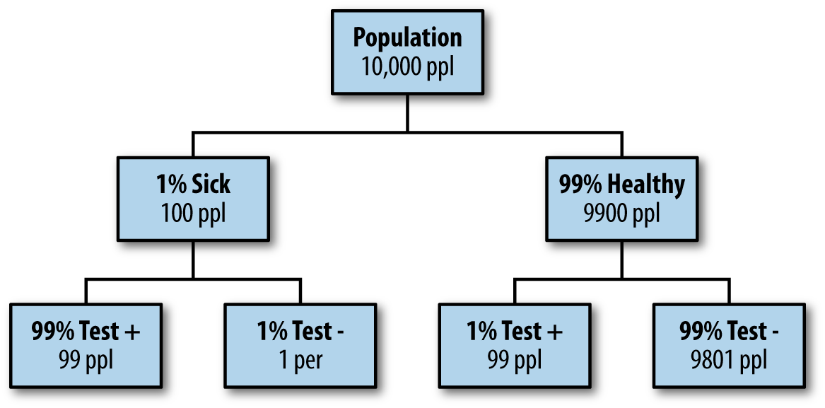
Figure 4-3. Tree diagram to build intuition
Let’s do it again using fancy notation so we’ll feel smart.
Recall from your basic statistics course that, given events and , there’s a relationship between the probabilities of either event (denoted and ), the joint probabilities (both happen, which is denoted ), and conditional probabilities (event happens given happens, denoted ) as follows:
Using that, we solve for (assuming ) to get what is called Bayes’ Law:
The denominator term, is often implicitly computed and can thus be treated as a “normalization constant.” In our current situation, set to refer to the event “I am sick,” or “sick” for shorthand; and set to refer to the event “the test is positive,” or “+” for shorthand. Then we actually know, or at least can compute, every term:
A Spam Filter for Individual Words
So how do we use Bayes’ Law to create a good spam filter? Think about it this way: if the word “Viagra” appears, this adds to the probability that the email is spam. But it’s not conclusive, yet. We need to see what else is in the email.
Let’s first focus on just one word at a time, which we generically call “word.” Then, applying Bayes’ Law, we have:
The righthand side of this equation is computable using enough pre-labeled data. If we refer to nonspam as “ham” then we only need compute p(word|spam), p(word|ham), p(spam), and p(ham) = 1-p(spam), because we can work out the denominator using the formula we used earlier in our medical test example, namely:
In other words, we’ve boiled it down to a counting exercise: counts spam emails versus all emails, counts the prevalence of those spam emails that contain “word,” and counts the prevalence of the ham emails that contain “word.”
To do this yourself, go online and download Enron emails. Let’s build a spam filter on that dataset. This really means we’re building a new spam filter on top of the spam filter that existed for the employees of Enron. We’ll use their definition of spam to train our spam filter. (This does mean that if the spammers have learned anything since 2001, we’re out of luck.)
We could write a quick-and-dirty shell script in bash that runs this, which Jake did. It downloads and unzips the file and creates a folder; each text file is an email; spam and ham go in separate folders.
Let’s look at some basic statistics on a random Enron employee’s email. We can count 1,500 spam versus 3,672 ham, so we already know and . Using command-line tools, we can also count the number of instances of the word “meeting” in the spam folder:
grep -il meeting enron1/spam/*.txt | wc -l
This gives 16. Do the same for his ham folder, and we get 153. We can now compute the chance that an email is spam only knowing it contains the word “meeting”:
Take note that we didn’t need a fancy programming environment to get this done.
Next, we can try:
-
“money”: 80% chance of being spam
-
“viagra”: 100% chance
-
“enron”: 0% chance
This illustrates that the model, as it stands, is overfitting; we are getting overconfident because of biased data. Is it really a slam-dunk that any email containing the word “Viagra” is spam? It’s of course possible to write a nonspam email with the word “Viagra,” as well as a spam email with the word “Enron.”
A Spam Filter That Combines Words: Naive Bayes
Next, let’s do it for all the words. Each email can be represented by a binary vector, whose th entry is 1 or 0 depending on whether the th word appears. Note this is a huge-ass vector, considering how many words we have, and we’d probably want to represent it with the indices of the words that actually show up.
The model’s output is the probability that we’d see a given word vector given that we know it’s spam (or that it’s ham). Denote the email vector to be and the various entries , where the indexes the words. For now we can denote “is spam” by , and we have the following model for i.e., the probability that the email’s vector looks like this considering it’s spam:
The here is the probability that an individual word is present in a spam email. We saw how to compute that in the previous section via counting, and so we can assume we’ve separately and parallelly computed that for every word.
We are modeling the words independently (also known as “independent trials”), which is why we take the product on the righthand side of the preceding formula and don’t count how many times they are present. That’s why this is called “naive,” because we know that there are actually certain words that tend to appear together, and we’re ignoring this.
So back to the equation, it’s a standard trick when we’re dealing with a product of probabilities to take the log of both sides to get a summation instead:
Note
It’s helpful to take the log because multiplying together tiny numbers can give us numerical problems.
The term doesn’t depend on a given email, just the word, so let’s rename it and assume we’ve computed it once and stored it. Same with the quantity . Now we have:
The weights that vary by email are the s. We need to compute them separately for each email, but that shouldn’t be too hard.
We can put together what we know to compute and then use Bayes’ Law to get an estimate of which is what we actually want—the other terms in Bayes’ Law are easier than this and don’t require separate calculations per email. We can also get away with not computing all the terms if we only care whether it’s more likely to be spam or to be ham. Then only the varying term needs to be computed.
You may notice that this ends up looking like a linear regression, but instead of computing the coefficients by inverting a huge matrix, the weights come from the Naive Bayes’ algorithm.
This algorithm works pretty well, and it’s “cheap” to train if we have a prelabeled dataset to train on. Given a ton of emails, we’re more or less just counting the words in spam and nonspam emails. If we get more training data, we can easily increment our counts to improve our filter. In practice, there’s a global model, which we personalize to individuals. Moreover, there are lots of hardcoded, cheap rules before an email gets put into a fancy and slow model.
Here are some references for more about Bayes’ Law:
-
“Idiot’s Bayes - not so stupid after all?” (The whole paper is about why it doesn’t suck, which is related to redundancies in language.)
-
“Naive Bayes at Forty: The Independence Assumption in Information”
Fancy It Up: Laplace Smoothing
Remember the from the previous section? That referred to the probability of seeing a given word (indexed by ) in a spam email. If you think about it, this is just a ratio of counts: where denotes the number of times that word appears in a spam email and denotes the number of times that word appears in any email.
Laplace Smoothing refers to the idea of replacing our straight-up estimate of with something a bit fancier:
We might fix and for example, to prevent the possibility of getting 0 or 1 for a probability, which we saw earlier happening with “viagra.” Does this seem totally ad hoc? Well, if we want to get fancy, we can see this as equivalent to having a prior and performing a maximal likelihood estimate. Let’s get fancy! If we denote by the maximal likelihood estimate, and by the dataset, then we have:
In other words, the vector of values is the answer to the question: for what value of were the data D most probable? If we assume independent trials again, as we did in our first attempt at Naive Bayes, then we want to choose the to separately maximize the following quantity for each :
If we take the derivative, and set it to zero, we get:
In other words, just what we had before. So what we’ve found is that the maximal likelihood estimate recovers your result, as long as we assume independence.
Now let’s add a prior. For this discussion we can suppress the from the notation for clarity, but keep in mind that we are fixing the th word to work on. Denote by the maximum a posteriori likelihood:
This similarly answers the question: given the data I saw, which parameter is the most likely?
Here we will apply the spirit of Bayes’s Law to transform to get something that is, up to a constant, equivalent to . The term is referred to as the “prior,” and we have to make an assumption about its form to make this useful. If we make the assumption that the probability distribution of is of the form for some and then we recover the Laplace Smoothed result.
Comparing Naive Bayes to k-NN
Sometimes and are called “pseudocounts.” Another common name is “hyperparameters.” They’re fancy but also simple. It’s up to you, the data scientist, to set the values of these two hyperparameters in the numerator and denominator for smoothing, and it gives you two knobs to tune. By contrast, k-NN has one knob, namely k, the number of neighbors. Naive Bayes is a linear classifier, while k-NN is not. The curse of dimensionality and large feature sets are a problem for k-NN, while Naive Bayes performs well. k-NN requires no training (just load in the dataset), whereas Naive Bayes does. Both are examples of supervised learning (the data comes labeled).
Sample Code in bash
#!/bin/bash## file: enron_naive_bayes.sh## description: trains a simple one-word naive bayes spam# filter using enron email data## usage: ./enron_naive_bayes.sh <word>## requirements:# wget## author: jake hofman (gmail: jhofman)## how to use the codeif[$#-eq1]thenword=$1elseecho"usage: enron_naive_bayes.sh <word>"exitfi# if the file doesn't exist, download from the webif![-e enron1.tar.gz]thenwget'http://www.aueb.gr/users/ion/data/enron-spam/preprocessed/enron1.tar.gz'fi# if the directory doesn't exist, uncompress the .tar.gzif![-d enron1]thentar zxvf enron1.tar.gzfi# change into enron1cdenron1# get counts of total spam, ham, and overall msgsNspam=`ls -l spam/*.txt|wc -l`Nham=`ls -l ham/*.txt|wc -l`Ntot=$Nspam+$Nhamecho$Nspamspam examplesecho$Nhamham examples# get counts containing word in spam and ham classesNword_spam=`grep -il$wordspam/*.txt|wc -l`Nword_ham=`grep -il$wordham/*.txt|wc -l`echo$Nword_spam"spam examples containing$word"echo$Nword_ham"ham examples containing$word"# calculate probabilities using bash calculator "bc"Pspam=`echo"scale=4;$Nspam/ ($Nspam+$Nham)"|bc`Pham=`echo"scale=4; 1-$Pspam"|bc`echoecho"estimated P(spam) ="$Pspamecho"estimated P(ham) ="$PhamPword_spam=`echo"scale=4;$Nword_spam/$Nspam"|bc`Pword_ham=`echo"scale=4;$Nword_ham/$Nham"|bc`echo"estimated P($word|spam) ="$Pword_spamecho"estimated P($word|ham) ="$Pword_hamPspam_word=`echo"scale=4;$Pword_spam*$Pspam"|bc`Pham_word=`echo"scale=4;$Pword_ham*$Pham"|bc`Pword=`echo"scale=4;$Pspam_word+$Pham_word"|bc`Pspam_word=`echo"scale=4;$Pspam_word/$Pword"|bc`echoecho"P(spam|$word) ="$Pspam_word# return original directorycd..
Scraping the Web: APIs and Other Tools
As a data scientist, you’re not always just handed some data and asked to go figure something out based on it. Often, you have to actually figure out how to go get some data you need to ask a question, solve a problem, do some research, etc. One way you can do this is with an API. For the sake of this discussion, an API (application programming interface) is something websites provide to developers so they can download data from the website easily and in standard format. (APIs are used for much more than this, but for your purpose this is how you’d typically interact with one.) Usually the developer has to register and receive a “key,” which is something like a password. For example, the New York Times has an API here.
Warning about APIs
Always check the terms and services of a website’s API before scraping. Additionally, some websites limit what data you have access to through their APIs or how often you can ask for data without paying for it.
When you go this route, you often get back weird formats, sometimes in JSON, but there’s no standardization to this standardization; i.e., different websites give you different “standard” formats.
One way to get beyond this is to use Yahoo’s YQL language, which allows you to go to the Yahoo! Developer Network and write SQL-like queries that interact with many of the APIs on common sites like this:
select * from flickr.photos.search where text="Cat"
and api_key="lksdjflskjdfsldkfj" limit 10
The output is standard, and you only have to parse this in Python once.
But what if you want data when there’s no API available?
In this case you might want to use something like the Firebug extension for Firefox. You can “inspect the element” on any web page, and Firebug allows you to grab the field inside the HTML. In fact, it gives you access to the full HTML document so you can interact and edit. In this way you can see the HTML as a map of the page and Firebug as a kind of tour guide.
After locating the stuff you want inside the HTML, you can use curl, wget, grep, awk, perl, etc., to write a quick-and-dirty shell script to grab what you want, especially for a one-off grab. If you want to be more systematic, you can also do this using Python or R.
Other parsing tools you might want to look into include:
- lynx and lynx --dump
-
Good if you pine for the 1970s. Oh wait, 1992. Whatever.
- Beautiful Soup
-
Robust but kind of slow.
- Mechanize (or here)
-
Super cool as well, but it doesn’t parse JavaScript.
- PostScript
Jake’s Exercise: Naive Bayes for Article Classification
This problem looks at an application of Naive Bayes for multiclass text classification. First, you will use the New York Times Developer API to fetch recent articles from several sections of the Times. Then, using the simple Bernoulli model for word presence, you will implement a classifier which, given the text of an article from the New York Times, predicts the section to which the article belongs.
First, register for a New York Times Developer API key and request access to the Article Search API. After reviewing the API documentation, write code to download the 2,000 most recent articles for each of the Arts, Business, Obituaries, Sports, and World sections. (Hint: Use the nytd_section_facet facet to specify article sections.) The developer console may be useful for quickly exploring the API. Your code should save articles from each section to a separate file in a tab-delimited format, where the first column is the article URL, the second is the article title, and the third is the body returned by the API.
Next, implement code to train a simple Bernoulli Naive Bayes model using these articles. You can consider documents to belong to one of C categories, where the label of the ith document is encoded as —for example, Arts = 0, Business = 1, etc.—and documents are represented by the sparse binary matrix , where indicates that the th document contains the th word in our dictionary.
You train by counting words and documents within classes to estimate and :
where is the number of documents of class c containing the th word, is the number of documents of class , is the total number of documents, and the user-selected hyperparameters and are pseudocounts that “smooth” the parameter estimates. Given these estimates and the words in a document x, you calculate the log-odds for each class (relative to the base class c = 0) by simply adding the class-specific weights of the words that appear to the corresponding bias term:
where
Your code should read the title and body text for each article, remove unwanted characters (e.g., punctuation), and tokenize the article contents into words, filtering out stop words (given in the stopwords file). The training phase of your code should use these parsed document features to estimate the weights , taking the hyperparameters and as input. The prediction phase should then accept these weights as inputs, along with the features for new examples, and output posterior probabilities for each class.
Evaluate performance on a randomized 50/50 train/test split of the data, including accuracy and runtime. Comment on the effects of changing and . Present your results in a (5×5) confusion table showing counts for the actual and predicted sections, where each document is assigned to its most probable section. For each section, report the top 10 most informative words. Also present and comment on the top 10 “most difficult to classify” articles in the test set.
Briefly discuss how you expect the learned classifier to generalize to other contexts, e.g., articles from other sources or time periods.
Sample R Code for Dealing with the NYT API
# author: Jared Lander## hard coded call to APItheCall<-"http://api.nytimes.com/svc/search/v1/article?format=json&query=nytd_section_facet:[Sports]&fields=url,title,body&rank=newest&offset=0&api-key=Your_Key_Here"# we need the rjson, plyr, and RTextTools packagesrequire(plyr)require(rjson)require(RTextTools)## first let's look at an individual callres1<-fromJSON(file=theCall)# how long is the resultlength(res1$results)# look at the first itemres1$results[[1]]# the first item's titleres1$results[[1]]$title# the first item converted to a data.frame, Viewed in the data viewerView(as.data.frame(res1$results[[1]]))# convert the call results into a data.frame, should be 10 rows by 3 columnsresList1<-ldply(res1$results,as.data.frame)View(resList1)## now let's build this for multiple calls# build a string where we will substitute the section for the first %s and offset for the second %stheCall<-"http://api.nytimes.com/svc/search/v1/article?format=json&query=nytd_section_facet:[%s]&fields=url,title,body&rank=newest&offset=%s&api-key=Your_Key_Here"# create an empty list to hold 3 result setsresultsSports<-vector("list",3)## loop through 0, 1 and 2 to call the API for each valuefor(iin0:2){# first build the query string replacing the first %s withSportandthesecond%swiththecurrentvalueofitempCall<-sprintf(theCall,"Sports",i)# make the query and get the json responsetempJson<-fromJSON(file=tempCall)# convert the json into a 10x3 data.frame andsaveittothelistresultsSports[[i+1]]<-ldply(tempJson$results,as.data.frame)}# convert the list into a data.frameresultsDFSports<-ldply(resultsSports)# make a new column indicating this comes from SportsresultsDFSports$Section<-"Sports"## repeat that whole business for arts## ideally you would do this in a more eloquent manner, but this is just for illustrationresultsArts<-vector("list",3)for(iin0:2){tempCall<-sprintf(theCall,"Arts",i)tempJson<-fromJSON(file=tempCall)resultsArts[[i+1]]<-ldply(tempJson$results,as.data.frame)}resultsDFArts<-ldply(resultsArts)resultsDFArts$Section<-"Arts"# combine them both into one data.frameresultBig<-rbind(resultsDFArts,resultsDFSports)dim(resultBig)View(resultBig)## now time for tokenizing# create the document-term matrix in english, removing numbers and stop words and stemming wordsdoc_matrix<-create_matrix(resultBig$body,language="english",removeNumbers=TRUE,removeStopwords=TRUE,stemWords=TRUE)doc_matrixView(as.matrix(doc_matrix))# create a training and testing settheOrder<-sample(60)container<-create_container(matrix=doc_matrix,labels=resultBig$Section,trainSize=theOrder[1:40],testSize=theOrder[41:60],virgin=FALSE)
Historical Context: Natural Language Processing
The example in this chapter where the raw data is text is just the tip of the iceberg of a whole field of research in computer science called natural language processing (NLP). The types of problems that can be solved with NLP include machine translation, where given text in one language, the algorithm can translate the text to another language; semantic analysis; part of speech tagging; and document classification (of which spam filtering is an example). Research in these areas dates back to the 1950s.
Get Doing Data Science now with the O’Reilly learning platform.
O’Reilly members experience books, live events, courses curated by job role, and more from O’Reilly and nearly 200 top publishers.

